Pepin, our Probabilistic Approximate Volume Counter

Let’s say you are allowed to have cubes in a 3-dimensional space that happens to be binary. In this space, x1, x2, and x3 are the axis, and for example the cube x1=0 is a cube that happens to have 4 points in it: 000, 001, 010, and 011. So far, so good. Now, let’s say we need to calculate the total volume of two cubes in this space. If they don’t intersect, it’s quite easy, we simply add their volumes. But what if they intersect? Now we need to compute their overlap, and subtract it from their sum of volumes. But there is a better way.

Probabilistic Approximate Volume Counting

Our new tool Pepin (code, paper) is based on the probabilistic approximate model counting algorithm by Meel, Vinodchandran, and Chakraborty (paper) that is so simple in principle yet so ingenious that even Donald Knuth got excited about it, recently writing a 15-page note and spending considerable amount of time on the algorithm.

So, what is this algorithm? Well, it’s so simple it’s almost funny. Basically, we keep randomly sampled points from the volume that we currently hold. At every moment we have a representative, evenly sampled set of points from the volume we currently have, and we know the sampling rate. You can think of the “sampling rate” as the approximate volume that each sample represents. So, if at any point we want to know the volume, we calculate number_of_points*(1/sampling_rate) and have the approximate volume. Kinda neat, no? So all we need is a randomly sampled set of points and a corresponding sampling rate. But how do we go about that?

Let’s say we are about to process the first cube (i.e. volume, could be any shape, actually, but cubes are simple). Our sampling rate is 1.0, we have 10 dimensions, and we have a limit of 10 samples in our bag. Let’s say the first cube is:

x1=0

Notice that this cube has 2^9 elements: 0000000000, 0000000001, … 0111111111. But that’s too many elements to hold, we only have space for 10 samples in the bag! We have to drop our sampling rate. The algorithm throws coins for each element in the volume (at first, a coin that has 1.0 probability of heads… funny coin!), and realizes that it won’t fit the sample bag. So it halves the sample rate (to 0.5) and throws the coins again. Realizes it doesn’t fit… halves the sample rate… and eventually will likely end up with a sampling rate of 1/2^6. That sample rate makes sense: it means 2^9/2^6 = 9 samples on average, which fits. Let’s say the algorithm flipped the coins, halved the sampling rate every time, and settled on a sampling rate of 1/2^6, and 9 samples.

Let’s see these samples. For readability, I’ll write the samples as 0110… which means x1=0, x2=1, x3=1, x4=0, etc.

Think of each of these points representing a volume of 2^6. The current estimate of the volume is 9*2^6 = 2^9.17 (instead of 2^9). So far so good. Now a new cube comes in. Let’s say this cube is:

x1=0, x1=1

This is the tricky part. What do we do? The algorithm is extremely simple: we throw away every sample that matches this cube, and then we sample the cube. Let’s throw away everything that matches, i.e. everything that starts with “01”:

Good. Now we sample the cube “x1=0, x1=1” with 1/2^6 probability. Time to take out our weird coin that has a 1/2^6 chance of winning! We toss this coin on every element in the cube, i.e. all 2^8 (since x0=1, x1=1 has 2^8 elements). We should get about 4 heads, but let’s say we got 3. Happens. Now, append these 3 to our neat little sample bag:

Nice. What just happened? Well, we got rid of the elements from the volume we were holding that were contained in the cube that we are processing. Then, we randomly sampled elements from the cube at our given sampling rate. If you think about it, this means that as long as we did everything uniformly at random, we are basically back to where we started. In fact, the 2nd cube could have been anything. It could have been completely outside of our current volume, or it could have partially intersected it. The game is the same. Running out of space? Just throw away each sample with probability half, and half your sampling rate! Here’s a visual representation what we would do in case the two cubes partially intersected:

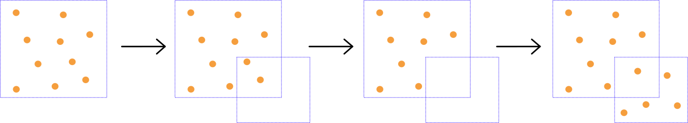
As the number of samples goes over the limit in our bag, we simply throw away each sample with 0.5 probability, and halve our sampling rate. This allows us to keep a fixed maximum number of samples, regardless of the size of the volume we are holding. For our example, we decided to limit ourselves to 10 samples, and got a pretty good estimate of the volume: 9*2^6 (=~2^9.17) instead of 2^9. One thing of note. This algorithm is not only approximate in the sense that we get something close to the actual solution, like 2^9.17. It’s also probabilistic in the sense that with a low probability, we get a complete garbage value. You can reduce the probability of getting a garbage value in a number of ways, though.

This algorithm is really powerful, because you could approximately count a 100-dimensional volume with thousands of cubes using less than 1MB of memory, and actually be pretty damn accurate, with a very low probability of getting a wrong value. Unsurprisingly, this is exactly what we do in our tool, Pepin.

The Tricks of Pepin

If you think about it, Pepin does nothing but: (1) holds a bunch of samples (2) deals with some large & small numbers (2^10000 is large, and 1/2^100000 is small), and (3) deals with probabilities. For dealing with small & large numbers, we used the GNU MP Bignum library, with all the standard tricks (pre-allocating memory & constants, etc), and for probabilities we use a number of tricks — sampling the binomial distribution is easy until you have to do it with t=2^100 and p=1/2^95. While dealing with probabilities was hard from a mathematical perspective, the really fun part for me was dealing with the sampling bag.

It turns out I wasn’t the only one who got sidetracked with the sampling bag: if you take a look at Knuth’s implementation, he goes into great detail about his datastructure, the Treap (honestly, that whole note by Knuth is quite a trip, you can see how his mind is racing). Anyway, back to the sampling bag. Firstly, the bag is just a matrix (with some rows sometimes empty) so we can store it either column or row-major. This is probably the first thing that comes to everyone’s mind as a computer science 101 trick. More interestingly, if one looks at the performance bottlenecks of the algorithm, it quickly becomes apparent that: (1) generating millions of bits of randomness for all the samples is expensive, and (2) writing all those samples to memory is expensive. So, what can we do?

The cool trick we came up with is what Knuth would call “late binding”, or we can call it lazy evaluation. Let’s keep to our original example: we first had the cube “x1=1”. We ran our coin-flip technique and found that we needed 9 samples (setting the sampling rate to 1/2^6), fine. But why do we really need all the bits of the samples? We don’t need them now! We may need them later — but since it’s all random anyway, we can generate them anytime, now or later! So, let’s generate 9 samples like this:

1*********
1*********
1*********
1*********
1*********
1*********
1*********
1*********
1*********

The “*” simply means this bit needs to be selected randomly. Now the cube “x1=1, x2=0” comes, which forces our hands, we have to know what the 2nd bit is: if it’s a “1” we have to throw the sample away, if it’s a “0”, we can keep it in. So we decide this bit now (not in the past, but now, when we need it), randomly:

00********
00********
00********
00********
01********
00********
01********
01********
00********

And now we can throw away the samples that match “x1=0, x2=1”, just like before. The sample bag is now:

00********
00********
00********
00********
00********
00********

We can now sample from the cube “x1=0, x2=1” randomly — again, notice we don’t need to know what the 3rd or 4th, etc. bits are. They can be decided later, when they are needed:

00********
00********
00********
00********
00********
00********
01********
01********
01********

Nice. Notice that this leads to exactly where we would have arrived anyway from a conceptual point of view. Except we (1) don’t need to generate as many random numbers and (2) if we can fill memory with “*” faster, then we can sample much faster.

In our implementation, we store values mem-packed, with 2 bits representing 0/1/*: for us, 00=0, 01=1, 11=*. This way, we can simply memset() with 1-s and fill it all up with “*”, a common occurrence. It probably won’t surprise anyone that of course we tried using a sparse matrix representation as well. It works very well for some problems. However, it depends what the exact problem is, and the performance degrades drastically for many problems. So the system uses dense representation by default. I’d be happy to merge a pull request that flips between sparse and dense depending on some density metric.

Obviously, I could not have done any of this alone. Pepin, the tool & paper, is by Divesh Aggarwal, Sourav Chakraborty, Kuldeep S. Meel, Maciej Obremski, and myself. Honestly speaking, it was wonderful to work together with all these amazing people.

Performance

At this stage, it should be obvious that it doesn’t even make sense to compare this tool to exact methods. The difference is mind-boggling. It’d be like racing a fighter jet against a rabbit. It’s a lot more fun to compare against other, existing approximate volume counting tools.

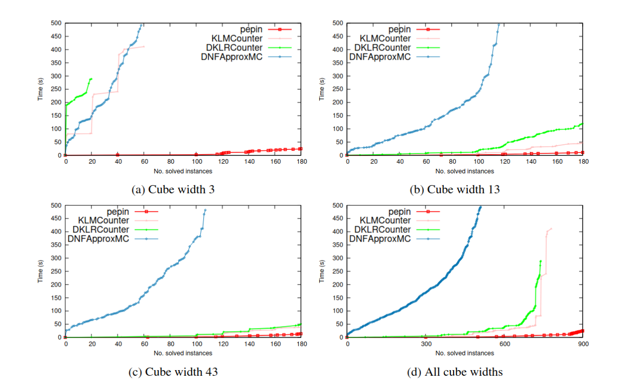
Above is a set of graphs of how Pepin performs against other approximate volume counting tools. Basically, it’s either way faster (easy 1000x speedup), or it’s a lot faster. Graph (c) is a bit misleading: for completeness, we included DNFApproxMC (PDF), which performs very poorly on these problems, and so Pepin seems to perform “as well as the others”. But, on closer examination:

Not really like the others: more like 3x faster than the others.

Potential Future Work

As mentioned above, a pretty straightforward (but not trivial) improvement would be to automatically switch to a sparse matrix representation. This would be akin to “making the horse run faster”, rather than inventing the steam engine, but hey, if it works, it works. Building a steam engine would be more like putting the whole algorithm into GPGPU and/or parallelizing it. It should be possible to rewrite this algorithm in a dynamic programming way, as it should be possible to combine sample bags and sampling probabilities (maybe not, I’m just an engineer). Then you can do divide-and-conquer. If you do that over a GPGPU that has 1000+ streaming cores, it could be possible to make this whole thing run 100x+ faster.

As engineers we like to over-engineer for performance, so it’s important to keep in mind that we are already hundreds of times faster than exact algorithms. Hence, perhaps it’d be more interesting to come up with interesting use-cases, rather than focusing on further improving speed. To keep with the horse analogy, it may be useful not to put the cart in front of the horse.

Closing Thoughts

Approximate volume counting is actually really cool. It takes the power of randomization and uses it to its own advantage to make something really difficult into something that one could explain a child. I have a feeling we could make a few beautiful graphics and teach this algorithm to 12 year olds. The sample-in-a-bag idea is so simple, yet so powerful. Actually, it’s also incredibly weird if you start going into the weeds of it. Like, what happens when the size of your bag is 1? It’s the kind of question that only Knuth would ask, and then answer with clarity and prowess that only one with deep mathematical insight can. I won’t even entertain the thought, but you can, if you read his notes and then work on his questions.

PS: Pepin was named after the rather eccentric character of the same name from Bohumil Hrabal‘s book Cutting It Short, also released as a film. Pepin in the book was inspired by Hrabal’s own uncle who came to visit his hometown for two weeks but stayed for 40 years. I think we have all been there.

Wonderings of a SAT geek

A blog about SAT solving and cryptography