Tag Archives: BCP

On variable renumbering

Variable renumbering in SAT solvers keeps a mapping between the external variable numbers that is visible to the users and the internal variable numbers that is visible the to the system. The trivial mapping that most SAT solvers use is the one-to-one mapping where there is no difference between outer and internal variables. A smart mapping doesn’t keep track of all data related to variables that have been set or eliminated internally, so the internal datastructures can be smaller.

Advantages

Having smaller internal data structures help in achieving a lower memory footprint and better cache usage.

The memory savings are useful because some CNFs have tens of millions of variables. If the solver uses the typical watched literal scheme, it needs 2 arrays for each variable. If we are using 64b pointers and 32b array sizes, it’s 32B for each variable, so 32MB for every million variable only to keep the watching literal array(!). I have seen people complaining that their 100M variable problem runs out of memory — if we count that right that’s 3.2GB of memory only to hold the watching literal array pointers and sizes, not any data at all.

As for the CPU cache benefits: modern CPUs work using cache lines which are e.g. 64B long on Intel Sandy Bridge. If half of the variables are set already, the array holding the variable values — which will be accessed non-stop during propagation — will contain 50% useless data. In practice the speedup achieved can be upwards of 10%.

The simple problems

One problem with having a renumbering scheme is that you need to keep track of which datastructure is numbered in which way. The easy solution is to renumber absolutely everything. This is costly, however, as the mapping has to change every once in a while when new variables have been set. In this case, if everything is renumbered, then the eliminated variables‘ data needs to be updated according to the new mapping every time. This might be quite significant. So, it’s best not to renumber that. Similarly, if disconnected component analysis is used, then the disconnected components’ saved solutions need to be renumbered as well, along with the clauses that have been moved to the components.

An approach I have found to be satisfying is to keep every dynamic datastructure such as variable states (eliminated/decomposed/etc.), variable values (True/False/Unknown), clauses’ literals, etc. renumbered, while keeping mostly static datastructures such as eliminated clauses or equivalent literal maps non-renumbered. This works very well in practice as it allows the main system to shuffle the mapping around while not caring about all the other systems’ data.

The hard problem

The above is all fine and dandy until bounded variable addition (BVA) comes to the scene. This technique adds new variables to the problem to simplify it. These new variables will look like new outer variables, which seems good at first sight: the system could simply print the solution to all variables except the last N that were added by BVA and are not part of the original problem. However, if the caller adds new variables after the call to solve(), what can we do? The actual variables by the caller and the BVA variables will be mixed up: start with a bunch of original variables, sprinkle the end with some BVA, then some original variables, then some BVA…

The trivial solution to this is to have another mapping, one that translates variable numbers between the BVA and non-BVA system. As you might imagine, this complicates everything. Another solution is to forcibly eliminate all BVA variables after the call to solve(), let the user add the new clauses, and perform BVA again. Another even more complicated solution is to keep track of the variables being added, then re-number all variables inside all datastructures to move all BVA variables to the end of the variable array. This is expensive but only needs to be done once after the call to solve(), which may be acceptable. Currently, CryptoMiniSat uses the trivial scheme. Maybe I’ll move to the last (and most complicated) system later on.

Conclusion

Variable renumbering is not for the faint of heart. Bugs become significantly harder to track, as all debug messages need to be translated to a common variable numbering or they make no sense at all. It’s also very easy to introduce bugs through variable renumbering. A truly difficult bug I had was when the disconnected component finder’s sub-solver renumbered its internal variables and when I tried to import some values from the sub-solver back to the main solver, I used the wrong variable numbers.
CryptoMinisat 3.1 released

CryptoMinisat 3.1 has been released. The short changelog is:

$ git diff cryptoms-3.0 cryptoms-3.1 --shortstat
 84 files changed, 3079 insertions(+), 2751 deletions(-)

The changes made were threefold. First, memory usage has been greatly reduced. This is crucial, because memory usage was over 7GB on certain instances. Secondly, the implication cache wasn’t very well-used and an idea that came to my mind greatly improved performance on most problems. Finally, time limiting of some inprocessing techniques on certain types of problems has been improved.

Memory usage reduction

On instances that produced a lot of long learnt clauses the memory usage was very high. These learnt clauses were all automatically linked in to the occurrence list and consequently took large amounts of memory, sometimes up to 10GB. On other instances, the original clauses were too numerous and too large, so putting even them into the occurrence list was too much. On these instances, variable elimination is not carried out (or carried out only later, when enough original clauses have been removed/shortened). To debug some of these problems, I wrote a fuzzer that generates extremely large problems with many binary and many long clauses, it’s available here as “largefuzzer”. It’s actually quite nice with many-many binary clauses so it also can fuzz the problems encountered with probing of extremely weird and large instances.

Implied literal usage improvement

CryptoMiniSat uses implied literals, i.e. caches what literals were propagated by each literal during probing. It then re-uses this information to subsume and/or strengthen clauses. This is kind of similar to stamping though uses more memory. It is actually useful to have alongside stamping, and I now do both — propagating DFS that stamping requires is expensive though updating cache during DFS is just as easy as during quasi-BFS.

The trick I discovered while playing around with cached implied literals is that if literal L1 propagates L2 and also !L2 then that means there are conceptually two binary clauses in the solver (!L1, L2), (!L1, !L2), so !L1 is TRUE. This is of course trivial, but I never checked for this. The question most would raise is: why would L1 propagate both L2 and !L2 and not fail? The answer is kind of tricky, but very interesting. Let’s say at one point, L1 propagates L2 due to a learnt clause, but that learnt clause is then removed. A new learnt clause is then later learnt, and with that learnt clause in place, L1 propagates !L2. Now, without caching, this would be ignored. Caching memorizes past conceptual binary clauses and re-uses this information.

This is not an optimization that only looks good on paper, it is very good to have. With this one optimization, I gained 5 instances from the SAT Comp’09 instances with a 1000s timeout (196 solved -> 201 solved). I can’t right now imagine how this could be done with stamping effectively, but that doesn’t mean it’s not possible. Though, according to my experience, stamping doesn’t preserve that much information over time as it’s being updated (renumbered) frequently while the cache is only improved over time, never shrunk. A possibility would be to have more than one stamp system and round-robin selecting them. However that would mean that sorting of clauses (for shrinking) would need to be done more than once, and sorting them is already relatively expensive. I sometimes feel that what stamping gains in memory it looses on sorting (i.e. processing time) and lower coverage (re-numbering).

More precise time-limiting

Martin Maurer has been kind enough to file a lot of bug reports about probing and variable elimination taking too much time, sometimes upwards of 150s when they should take around 20-30s maximum. While investigating, it tuned out that the problem was very weird indeed. While trying to eliminate or probe one variable the time for that one variable took upwards of 100s. This was completely unexpected as the code only checked for timeouts on a per-variable basis. In the end, the code had to be improved to track time on an intra-variable basis in both systems. While at it, I also added intra-variable time-tracking to implicit clause subsumption and strengthening too. So, over-times should less prevalent from now on. As an interesting side-note, time-limiting on probing is now so fine-grained that a 32-bit unsigned integer would overflow within 15s if used as the time-tracker.

On benchmark randomization

As many of you have heard, the SAT Competition for this year has been announced. You can send in your benchmarks between the 12th and the 22nd of April, so get started. I have a bunch of benchmarks I have already submitted about 2 years ago, still waiting for any reply from those organizers — but the organizers are different this year, so fingers crossed.

What I want to talk about today is benchmark randomization. This is a very-very touchy topic. However, I fear that it’s touchy for the wrong reasons, and so I think it’s important to talk about it in detail.

What is benchmark randomization?

Benchmark randomization is when a benchmark that is submitted is shuffled around a bit. There are many ways to shuffle a problem, and I will discuss this in a bit, but the point is that the problem at hand that is described by the benchmark CNF should not be changed, or changed only in a very-very minor way, such that everyone agrees that it doesn’t affect the core problem itself as described by the CNF.

Why do we need shuffling?

We need shuffling because simply put, there aren’t enough good benchmarks and so the benchmarks of yesteryear (and the year before, and before, and…) re-appear often. This would be OK if SAT solvers couldn’t be tuned to solving specific problems faster. Note that I am not suggesting that SAT solvers are intentionally manipulated to solve specific problems faster by unscrupulous researchers. Instead, the following happens.

Unintentional random seed improvements

Researchers test the performance of their SAT solvers on specific instances and then tune their solvers, testing the performance again and again on the same instances to check if they have improved performance. Logically this is the best way to test and improve performance: use the same well-defined test-set all the time for meaningful comparison. Since the researcher wants to use the instances that he/she thinks is the current use-case of SAT solvers, he naturally uses the instances of SAT competitions, since those are representative. I did and still do the same.

So, researchers add their idea to a SAT solver, and test. If the idea is not improving things then some change is made and tested again. Since modern CDCL SAT solvers behave quite randomly, and since any change in the source code changes the behaviour quite significantly, a small change in the source code (tuning of a parameter, for example) will change the behaviour. And since the set of problems tested on is fixed, there is a chance that more problems will be solved. If more are solved, the researcher might correctly interpret this as a general improvement, not specific to the problem set. However, it may very well be generic, it is also specific.

The above suggests that the randomness of the SAT solver is completely unintentionally tuned to specific problems — a subset of which will appear next year in the competition.

Easy fixes

Since there aren’t enough benchmark problems, and in particular some benchmark types are rare, I suggest to fix the unintentional tuning of solvers to specific problems by changing the benchmarks in minor ways. Here is a list, with an explanation why I think it’s OK to perform the manipulation:

  1. Propagate variables. Unitary clauses are often part of benchmarks. Propagating some of these, some recursively, gives quite a bit of problem space variation. Propagation is performed by every CDCL SAT solver, and I think many would be  surprised if it didn’t help SAT solvers that worked differently than  current SAT solvers. Agreeing on performing partial propagation is something that shouldn’t be too difficult.
  2. Renumber variables. For some variable X that is not used (or is fixed to a value that has been propagated), every variable that is higher than X is decremented by one, and the CNF header is fixed to reflect this change.  Such a minor renumbering may be approved by every researcher as something that doesn’t change the problem or its structure. Note that if  partial propagation is performed there should be quite a number of variables that can be removed. Renumbering some, but not others is a way to shuffle the problem. A more radical way of renumbering variables would be to completely shuffle them, however that would change the way the problem is described in quite a radical way, so some would correctly object and it’s not necessary anyway.
  3. Replace equivalent literals. Perform strongly connected component analysis and replace equivalent literals. This has been shown to significantly improve performance and I have never seen a case where it doesn’t. Since equivalent literal replacement can be performed with a lot of freedom, this is quite a bit of shuffling space. For example, if v1=v2=v3, then any of the v1, v2, v3 can be the one that replaces the rest in the CNF. Picking one randomly is a way to shuffle the instance

There are other ways of shuffling, but either they change the instance too much (e.g. blocked clause removal), or can be undone quite easily (e.g. shuffling the order of the clauses). In fact, (3) is already quite a touchy issue I think, but with (1) and (2) all could agree on. Neither requires the order of the literals or the order of the clauses to change — some clauses (e.g. unitary ones) and literals (some of those that are set) would be removed, but that’s all. The problem remains essentially unchanged such that most probably even the original problem author would easily recognize it. However, it would be different from a SAT solver point of view: these changes would change the random seed of the solver, forcing the solver to behave in a way that is less tuned to this specific problem instance.

Conclusion

SAT solvers are currently tuned too much to specific instances. This is not intentional by the researchers, however it still affects the results. To obtain better, less biased results we should shuffle the problem instances we have. Above, I suggested three ways to shuffle the instances in such a way that most would agree they don’t disturb or change the complexity of the underlying problem described by the instance. I hope that some of these suggestions will be employed, if not this year then for next year’s SAT competition such that we could reach better, more meaningful results.

Failed literal probing and UIP

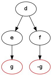
I have just realised that CryptoMiniSat, having won a number of medals, does one of the most basic things, failed literal probing, all wrong. Let me tell you why it’s all wrong. In essence, failed literal probing is trivial. We enqueue a fact, such as a, and then propagate it. If this fails, i.e. if two opposing facts such as g and -g are derived, we know that a cannot be true, so we set -a. Easy. Or maybe not so easy.

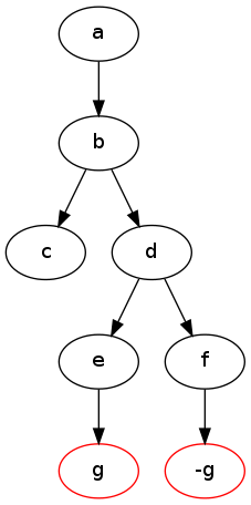
The devil is in the details, so let’s see how we derived both g and -g from a. Let’s assume that we have the following set of binary clauses:
-a V b
-b V c
-b V d
-d V e
-d V f
-e V g
-f V -g

which, from the point of view of a is best described as the graph:

Propagating "a", deriving both "g" and "-g"

The problem is, that if we only derive -a from this graph, we end up with only that one literal set, because -a doesn’t propagate anything on the clauses. This is quite sad, because, in fact, we could derive something stronger. From the graph it is evident that setting d would have failed: the graph would simply have its upper part cut away completely, but the lower part, including the derivation of both g and -g would still stand:

Deriving both "g" and "-g" from "d"

What is special about node d? Well, it’s where the 1st UIP, the first unique implication point, lies. And it is quite simple to see that -d is in fact the strongest thing we can derive from this graph. It’s much stronger than simply -a, because setting -d propagates on the clauses, giving -b,-a, setting three variables instead of one, including -a. An interesting observation is the following: deriving -b is the 2nd UIP, and deriving -a is the last UIP. In other words, at least in this most simple case, 1st UIP is in fact the strongest, and 2nd, 3rd.. last UIP are less strong in strict order.

Let me remark on one more thing about failed literal probing. Once failed literal probing has been done on literal x and it visited the node set N, there is no need to try to do failed literal probing on any nodes in N, since they cannot possibly fail. Although the failing of a literal can have consequences on the failing of other literals, if we ignore this side-effect, we could speed up failed literal probing by marking literals already visited, and only carrying out failed literal probing on ones that haven’t been marked. This is really trivial, but I haven’t been using it :S

I am quite sure that some advanced SAT solvers (such as lingeling) do all of the above things right. It’s probably only CryptoMiniSat that fails miserably :)

Note: there is a subtle bug with marking literals visited as “OK”. If two different subgraphs could fail, but we abort on the first one, then we might mark a literal OK when in fact it isn’t. It is therefore easiest not to mark any literals if the probe failed (which is very rare).

Understanding Implication Graphs

Having won the SAT Race with CryptoMiniSat, I think I can now confess that I still don’t understand conflict generation. So today, I sat down and I tried to understand it. The result is some fun code, a lot of reading, and great pictures. Let me share with you these auto-generated graphs — the generator will be released with CMSat 3.0.0, so you will be able to generate them, too. These graphs show something called an ‘implication graph’, which is nothing more than a graphical way to show how propagations were made by the reasoning engine. For instance, if variable x1 and x2 are both FALSE, then clause ‘x1 V x2 V x3’ will force x3 to be TRUE to satisfy the clause. Okay, so much for talk, let’s see the graphs!

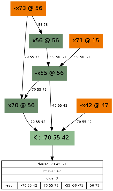
Our first implication graph had a clause “-70 55 42” (light green box) that caused a conflict — that is to say, somehow the variable setting {x70=TRUE, x55=FALSE, x42=FALSE} was set, the SAT solver realised that this is wrong, and something has to be done. Let’s look at what lead here! Guesses are coloured orange here, so it seems we made the following guesses during our SAT solving: x71=TRUE, x73 = FALSE, x42=FALSE. Now, we could just say, oh, well, setting x73 to FALSE was a dumb idea, just reverse that guess, and be done with it. That’s the easy (and the fast) way, but we are less lazy than that and we want to understand the reasons. So we do something called the conflict analysis to find something called an asserting clause that will not only let us reverse the guess x73=FALSE, but will also give the SAT solver a reason why that is a necessary assignment given its previous guesses and their consequences.

Consequences in the graph are coloured dark green, and there are exactly 3 of them: x70=TRUE, x55=FALSE and x56=TRUE. Each of these is a consequence of a clause that is in the SAT solver, marked on the edge(s) leading to it. For example, x56 is set to TRUE, because of the guess x73=FALSE and the clause “x56 V x73” marked on the edge leading to x56. A consequence that has one edge leading to it was propagated by a 2-long clause, a consequence that has 2 edges leading to it was propagated by a 3-long clause (e.g. consequence “x70=TRUE”, propagated by “x70 V x55 V x73”), etc. Okay, so how do we get to the reason? Well, we start out with the conflict, the clause “-x70 V x55 V x42” (at the bottom), and we do resolutions with this clause, going bottom up. We do as many resolutions as needed to reach the first UIP (also called “articulation vertex” or “dominator”), which is a unique point on the graph through which all paths go through from the highest decision level guess, in this case x73=FALSE, at decision level 56 (noted with a @56). If you take a look, the paths from x73=FALSE diverge from the very first point onwards, and there is no single point where they converge again. This means that the (first and only) dominator will be x73=FALSE itself, and we have to resolve with all clauses on the path:

  1. Start with clause “-x70 V x55 V x42”
  2. Resolve with clause “x70 V x55 V x73”
  3. Resolve with clause “-x55 V-x56 V -x71”
  4. Resolve with clause “x56 V x73”

This list is noted on the bottommost box’s lowest entry. When we resolve with these clauses, we are actually doing cuts on the graph, like this:

My drawing capabilities aren’t exactly great, but you can see that the cuts are successively higher and higher, until we reach the cut that has on its outer part the literals -x73, x71 and -x42. Unsurprisingly, exactly the inverse of these literals are what make up the final conflict clause. Now, if we unroll the implications until decision level 47 (but not the guess x42=FALSE), then with this clause added, variable x73 will propagate to TRUE automatically, essentially reversing the wrong guess — but also giving a reason why it needs to be reversed.

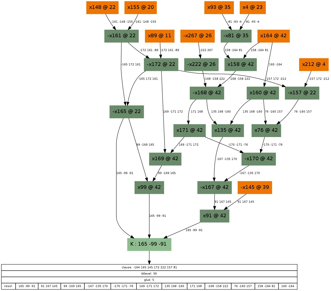
If you enjoyed the previous graph, here is another to entertain you further:

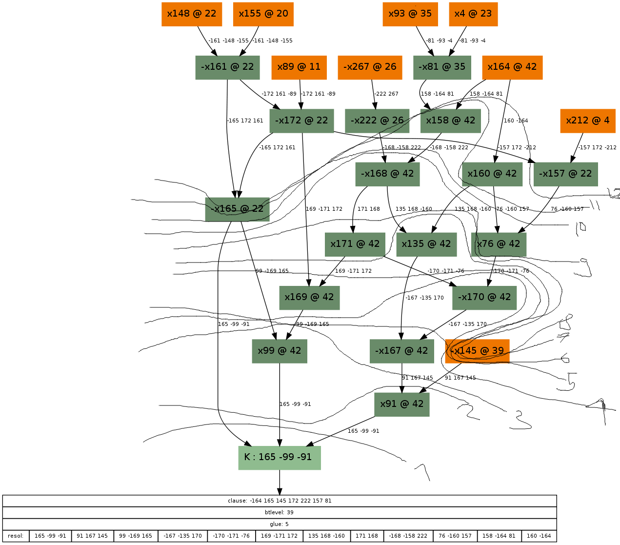
And its corresponding, not too obvious solution:

Note that I was too lazy to draw cuts 10, 11 and 12 around the assignment x145=FALSE (at decision level 39). The UIP in this case is again at the decision variable, x164. If you are still interested, here are some other examples:

PS: Thanks to George Katsirelos for his help understanding this (disclaimer: all faults belong to me alone).