Category Archives: SAT

Checking Uniform-Like Samplers

Uniform sampling is pretty simple: there are a set of solutions to a set of equations, and I want you to give me N solutions uniformly at random. Say, I have a set of equations that only has the solutions x=1…6, and I ask you to give me solutions uniformly at random. In this case, if the system is not cheating, it should give me solutions exactly like a random dice would give: 1..6, each with the same probability of 1/6. Now, if you give me nothing but 1’s I’d be slightly confused, and eventually would think you may be trying to cheat.

Uniformity is useful not only in gambling, but also e.g. if you want to make sure to cover a good chunk of the potential states in a system. Say, your equations describe how a program can run. Now, uniform solutions to these equations will be examples of the state space of your program. If you want to check that your system is in most cases doing the right thing, you can ask for uniform solutions at random and check the states for inconsistencies or unexpected behaviors.

Uniform Sampling of CNFs

One type of equations that is quite popular is to have all variables boolean (i.e. True/False), and equations being nothing but an “AND of ORs”, i.e. something like: “(a OR b) AND (b OR c OR d) AND (-f OR -g)”. These types of equations, also known as CNF, can express quite complicate things, e.g. (parts of) computer programs, logical circuits (e.g. parts of CPUs), and more. What’s nice about CNF is that there are many different tools to convert your problem language into CNF.

Given CNF as the intermediate language, all you need to do is run a uniform sampler on the CNF, and interpret the samples given your transformation. For example, you could translate your Ethereum cryptocurrency contract into QF_BV logic and blast that to CNF using e.g. the STP solver. Then you can get uniform random examples of the execution of your cryptocurrency contract using e.g. UniGen.

There are many different samplers for CNFs, and they mostly fall into two categories: ones that give guarantees and are hence truly uniform, and ones that don’t give guarantees and therefore fall into what we’ll call uniform-like samplers. These latter samplers tend to be significantly faster than truly uniform samplers, however, they can, and sometimes do, give non-uniform samples. I personally help maintain one truly uniform sampler, UniGen (PDF), and one uniform-like sampler, CMSGen (PDF). Other popular truly uniform samplers include KUS (PDF) and SPUR (PDF).

Catching Uniform-Like Samplers: Barbarik

If I give you a sampler and ask you to tell me if it’s truly uniform or simply uniform-like, what should you do? How should we distinguish one from the other, without looking into the internals of the system? It turns out that this is not a simple question to answer. It is very reasonable to assume that there are e.g. 2^200 solutions, so e.g. trying to prove that a sampler is uniform by saying that it should only output the same sample twice rarely is not really meaningful. In this latter case, you’d need to get approx 2^100 samples from a truly uniform sampler before it will likely give two colliding samples. While a uniform-like sampler may collide at e.g. only 2^60 (i.e. a trillion times earlier), that’s still a lot of computation, and only a single data point.

Doing this efficiently is the question that was on the minds of the authors of Barbarik. Basically, their idea was the following: take a CNF, remove all solutions but two, and blow up these two solutions into equally many solutions each. Say, you find two solutions to a CNF, one BLUE and one RED. Barbarik will take BLUE, make 100 blue balls out of it, and take RED, and make 100 red balls out of it. Then, it will give the CNF with the 200 solutions, half blue, half red, to the sampler under test. Then it asks the sampler to give it a bunch of balls. We of course expect approx 50%-50% red-blue distribution of balls from a truly uniform sampler.

Barbarik fails a solver if it is gives a distribution too far away from the 50%-50% we’d expect. Barbarik runs this check many times, with different example blue/red solutions that are “blown up” to multiple solutions. Given different base CNFs, and many tries, it is possible to differentiate the good from the bad… most of the time:

If you take a look at the table above, QuickSampler and STS, both uniform-like samplers, are rejected by Barbarik given 50 different CNFs. In contrast, UniGen survives all 50 tests with flying colors. Notice, however, that CMGen also survived all tests.

The Birth of CMSGen

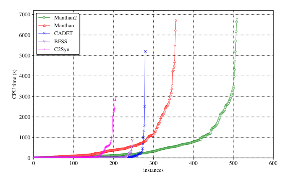
When Barbarik was being created, I was fortunate enough to be present, and so I decided to tweak my SAT solver, CryptoMiniSat purely using command-line parameters, until Barbarik could not distinguish it from a truly uniform sampler. This, in my view, showcased how extremely important a test system was: I actually had a bug in CryptoMiniSat’s randomization that Barbarik clearly showed and I had to fix to get higher quality samples. We called the resulting uniform-like sampler CMSGen, and it was used in the function synthesis tool Manthan (PDF), that blew all other function synthesis system out of the water, thanks to its innovative design and access to high quality, fast samples from CMSGen:

Notice that within 200 seconds Manthan outperformed all other function synthesis systems, even if we give the other system 7000 seconds to work with. If you are interested in the details of this crazy improvement over previous state-of-the-art, check out the slides here or the video here (these are all work of my coworkers, I am not an author).

While CMSGen was clearly fast and powerful, it bothered me endlessly that Barbarik couldn’t demonstrate that it wasn’t a truly uniform sampler. This eventually lead to the development of ScalBarbarik.

The Birth of ScalBarbarik

Since CMSGen passed all the tests of Barbarik, we had to come up with a new trick to distinguish it from truly uniform samplers. ScalBarbarik‘s (PDF) underlying system is still the same as Barbarik: we take a CNF, take 2 samples from it, and blow both of these samples up to a certain number. However, how we blow them up is where the trick lies. Before, they were both blown up the same way into solutions that are equally easy/hard to find. However, this time around, we’ll make one of the solution types much harder to find than the other. For this, we’ll use Vegard Nossum’s SHA-1 CNF generator (PDF) to force the system to reverse a partial, reduced-round SHA-1 hash, with some fixed inputs & outputs. This allows us to both change the complexity of the problem and the number of solutions to it rather easily.

While one set of solutions will be hard to find, the other ones will be trivial to find — if one special variable is set to TRUE, the finding a set of solutions is trivial But when it’s set to FALSE, the system has to reverse a reduce-round SHA-1. The logic behind this is that the uniform-like systems will likely be finding the easy solutions with much higher probability than the hard solutions, so they will sample much more unevenly. Indeed that’s the case:

Note that as the hardness parameter is increased, CMSGen is rejected more and more often, and eventually it’s rejected for all CNFs. Also interesting to note is that QuickSampler and STS get both rejected, as before, but this time around, STS gets rejected for all 50 CNFs, rather than for only 36 out of 50. In other words, ScalBarbarik is overall a stronger/better distinguisher.

Conclusions

With the birth of Barbarik, a set of uniform-like testers were shown to be less than ideal, and a new, more robust near-uniform sampler was born, CMSGen. But as a the gauntlet has been throw down by CMSGen, a new tool emerged, ScalBarbarik, to help find the non-truly uniform samplers. With this cycle in mind, I hope that new, more elaborate, and higher-quality uniform-like samplers will emerge that will be able to beat ScalBarbarik at its own game, improving the quality of the sampling while maintaining the speed advantage that uniform-like samplers enjoy over truly uniform samplers. With better uniform-like sampling tools, hopefully we’ll be able to make headway in automated test case generation (imagine having it as part of all development IDEs), higher performance function synthesis, and hopefully even more diverse areas of interest for the general public.

CMSGen, a Fast Uniform-Like Sampler

Uniform sampling is a problem where you are given a solution space and you have to present solutions uniformly, at random. In some cases, this is quite simple, say, for the lotto. Just pick 5 random numbers from a box and we are done! For the lotto the solution space is very easy to generate. However, when there are constraints on the solution space, it starts to get tricky.

Let’s say that I have a function I want to test, but the input to the function has some real-world constraints like e.g. the 1st parameter must be larger than the second, the 2nd parameter must be divisible by the 3rd etc. If I want to test that this function operates correctly, one way to do it is to generate 100 uniformly random inputs that don’t violate any of the constraints, run the function, and see if all is OK. For this, I need a fast way of generating uniform samples given the constraints on the solution space.

Sampler speed vs. accuracy

There have been many samplers proposed in the literature. I personally have worked on one called UniGen, a guaranteed approximate probabilistic sampler, meaning that it’ll give approximately uniform samples most of the time, and we have a proof to back this up. It’s a great sampler and will work very fast on many instances. However, for really complex solution spaces, it can have trouble. Say, you want to generate interesting test inputs for your deep learning algorithm. Deep neural networks tend to be extremely complex when translated to binary constraints, so UniGen will likely not be fast enough. It would give very good quality samples (i.e. properly uniform samples), but if it’s too slow, we may want to exchange quality of samples for speed of generation.

There are two well-known samplers that are supposed to generate uniform samples on complex solution spaces, QuickSampler (code), and STS (code), but give no guarantees, let’s call these “uniform-like” samplers. Unfortunately, the paper by Chakraborty et al and its resulting code Barbarik showed that these uniform-like samplers are highly non-uniform. Barbarik is a pretty neat idea that basically constructs solution spaces with known solution distributions and then asks the sampler to generate uniform samples. Knowing the solution space, Barbarik can then verify how non-uniform the sampler is. Imagine having a box with 1000 balls, half of them blue and the other half green. Now if I ask the sampler to give me 50 balls at random, and all of them are green, I’d be a bit surprised to say the least. It’d be like the 5-lottery having the same numbers 3 times in a row. Possible, but… not very likely. If I do this experiment 100 times, and I always get 50 green balls, it’s fair to conclude that the sampler is not uniform.

Our new uniform-like sampler, CMSGen

Given an effective tester, Barbarik, we (Priyanka Golia, Sourav Chakraborty, Kuldeep S. Meel, and myself) thought perhaps we can follow the nowadays very successful test-driven development (TDD) methodology. All we have to do is to make our sampler pass the test of Barbarik, while being at least as fast as STS/QuickSampler, and we’ll be good to go. In fact, given Barbarik, it only took about a week of playing around with CryptoMiniSat’s options to beat both STS and QuickSampler in both accuracy and speed. This speaks volumes to how important it is to have a robust, reliable, and fast testing framework that can give immediate feedback about the quality of samples generated.

Our new uniform-like sampler, based on CryptoMiniSat, is called CMSGen (research paper here), and effectively takes CyrptoMiniSat and applies the following set of changes, through pre-set command line options:

  • Pick polarities at random. Normally, SAT solvers use polarity caching scheme, but of course we want uniform samples over all the search space, so we need to pick polarities at random.
  • Branch on variables at random. Normally, SAT solver branch on variables that will most likely lead to a conflict to maximize search efficiency (the VSIDS heuristic). However, we want to explore the solution space as evenly as possible, and so we want to approach the solution space from as many angles as possible. If you think about the search space as an N-dimensional binary cube, then we are trying to approach this cube as any ways as possible.
  • Turn off all pre- and inprocessing. Pre and inprocessing in SAT solvers are used to minimize the instance, transforming it into something easier to solve, e.g. through Bounded Variable Elimination. We later reconstruct a viable solution based on the solution to the transformed instance. However, the transformed instance may (and often will!) have a very different solution space. We cannot have that, so we must turn this off. To be fair, some pre- and inprocessing could be left intact, e.g. subsumption and self-subsuming elimination, perhaps a future paper :)
  • Restart at static intervals. Restarts are nowadays often dynamic in modern SAT solvers, or even if not dynamic, then follow a non-regular pattern. However, that could disturb how we find solution. Imagine, let’s say that solutions with variable A set to TRUE are very easy to find, but solutions with FALSE are very hard to find. What will happen? Well, in restarts where A was randomly set to TRUE, we’ll always quickly find a solution and output it. But for restarts when A was randomly set to FALSE, the system would struggle to find a solution, and after some conflicts, it will simply restart into a status where hopefully A is set to TRUE, and it can find a solution again. It is quite clear to see that this will lead to serious issues with sampling quality. Hence, we set an adjustable but static restart interval of 100 conflicts, with higher values typically leading to more uniform samples.

Performance of CMSGen

Performance of the system is on the ridiculous scale in comparison with other samplers:

When it comes to 2-wise coverage, i.e. the quality of samples, the data speaks for itself (note, UniGen is missing here because it was too slow):

Note that between STS and QuickSampler, STS is both the more uniform sampler, but also the slower one. CMSGen overcomes this limitation: it’s both faster than QuickSampler, and more uniform than STS.

And of course, the Barbarik tester gives “Accept” on CMSGen much more often than on STS or QuickSampler:

Conclusion

If you need non-guaranteed uniform but fast sampling, I’d go and try out CMSGen. It’s really a completely different beast. It’s not a guaranteed uniform sampler, but it’s incredibly effective. In fact, it’s so effective and works so well, it took me a full year to figure out how best to generate problems for it where it wouldn’t be uniform. But that’s another paper, and another blog post! In the meantime, the sampler is here, go check it out!

CryptoMiniSat 5.8.0 Released

After many months of work, CryptoMiniSat 5.8.0 has been released. In this post I’ll go through the most important changes, and how they helped the solver to be faster and win a few awards, among them 1st place at the SAT incremental track, 3rd place SAT Main track, and 2nd&3d place in the SMT BitVector tracks together with the STP and MinkeyRink solvers.

Gauss-Jordan Elimination

First and foremost, Gauss-Jordan elimination at all levels of the search is now enabled by default. This is thanks to the work detailed in the CAV 2020 paper (video here). The gist of the paper is that we take advantage of the bit-packed matrix and some clever bit field filters to quickly check whether an XOR constraint is propagating, conflicting, or neither. This, and a variety of other improvements lead to about 3-10x speedup for the Gauss-Jordan elimination procedure.

With this speedup, the overhead is quite small, and we enable G-J elimination at all times now. However, there are still limits on the size of the matrix, the number of matrices, and we disable it if it doesn’t seem to improve performance.

As a bit of reflection: our original paper with Nohl and Castelluccia on CryptoMiniSat, featuring Gauss-Jordan elimination at all levels of the search tree was published at SAT 2009. It took about 11 years of work, and in particular the work of Han and Jiang to get to this point, but we finally arrived. The difference is day and night.

Target Phases

This one is really cool, and it’s in CaDiCaL (direct code link here) by Armin Biere, description here (on page 8). If you look at the SAT Race of 2019, you will see that CaDiCaL solved a lot more satisfiable problems than any other solver. If you dig deep enough, you’ll see it’s because of target phases.

Basically, target phases are a variation of phase saving, but instead of saving the phase all the time when backtracking, it only saves it when backtracking from a depth that’s longer than anything seen before. Furthermore, it is doing more than just this: sometimes, it picks only TRUE, and sometimes it picks only FALSE phase. To spice it up, you can keep “local deepest” and “global deepest” if you like, and even pick inverted phases.

It’s pretty self-explanatory if you read this code (basically, just switching between normal, target, inverted, fixed FALSE, fixed TRUE phases) and it helps tremendously. If you look at the graphs of the SAT 2020 competition results (side no. 19 here) you will see a bunch of solvers being way ahead of the competition. That’s target phases right there.

CCAnr Local Search Solver

CryptoMiniSat gained a new local search solver, CCAnr (paper here) and it’s now the default. This is a local search solver by Shaowei Cai who very kindly let me add his solver to CryptoMiniSat and allowed me to add him as an author to the version of CryptoMiniSat that participated in the SAT competition. It’s a local search solver, so it can only solve satisfiable instances, and does so by always working on a full solution candidate that it tries to “massage” into a full solution.

Within CryptoMiniSat, CCAnr takes the starting candidate solution from the phases inside the CDCL solver, and tries to extend it to fit all the clauses. If it finds a satisfying assignment, this is emitted as a result. If it doesn’t, the best candidate solution (the one that satisfies the most clauses) is saved into the CDCL phase and is later used in the CDCL solver. Furthermore, some statistics during the local search phase are saved and then injected into the variable branching heuristics of the CDCL solver, see code here.

Hybrid Variable Branching

Variable branching in CryptoMiniSat has always been a mix of VSIDS (Variable State Independent Decaying Sum, paper here) and Maple (multi-arm bandit based, paper here) heuristics. However, both Maple and VSIDS have a bunch of internal parameters that work best for one, or for another type of SAT problem.

To go around the issue of trying to find a single optimal value for all, CryptoMiniSat now uses a combination of different configurations that is parsed from the command line, such as: “maple1 + maple2 + vsids2 + maple1 + maple2 + vsids1” that allows different configurations for both Maple and VSIDS (v1 and v2 for both) to be configured and used, right from the command line. This configuration system allows for a wider variety of problems to be efficiently solved.

Final Remarks

CryptoMiniSat is now used in many systems. It is the default SAT solver in:

I think the above, especially given their track record of achieving high performance in their respective fields, show that CryptoMiniSat is indeed a well-performing and reliable workhorse. This is thanks to many people, including, but not limited to, Kuldeep Meel, Kian Ming A. Chai, Trevor Hansen, Arijit Shaw, Dan Liew, Andrew V. Jones, Daniel Fremont, Martin Hořeňovský, and others who have all contributed pull requests and valuable feedback. Thanks!

As always, let me know if you have any feedback regarding the solver. You can create a GitHub issue here, and pull request here. I am always interested in new use-cases and I am happy to help integrate it into new systems.

SAT Solvers as Smart Search Engines

Satisfiability problem solvers, or SAT solvers for short, try to find a solution to decidable, finite problems such as cryptography, planning, scheduling, and the like. They are very finely tuned engines that can be looked at in two main ways . One is to see them as proof generators, where the SAT solver is building a proof of unsatisfiability as it runs, i.e. it tries to prove that there is no solution to the problem. Another way is to see SAT solvers as smart search engines. In this blog post, I’ll take this latter view and try to explain why I think intermediary variables are important. So, for the sake of argument, let’s forget that SAT solvers sometimes restart the search (forgetting where they were before) and learn clauses (cutting down the search space and remembering where not go again). Let’s just pretend all they do is search.

Searching

The CryptoMiniSat SAT solver used to be able to generate graphs that show how a search through the search space went. Search spaces in these domains are exponential in size, say, 2^n in case there are n variables involved. I don’t have the search visualization code anymore but below is an example of such a search tree. The search starts at the very top not far from the middle, it descends towards the bottom left, then iteratively backtracks all the way to the top, and then descends towards the bottom right. Every pentagon at the bottom of a line is a place where the SAT solver backtracked. Observe that it never goes all the way back to the top — except once, when the top assignment needs to be flipped. Instead, it only goes back some way, partially unassigning variables. The bottom right corner is where the solution is found after many-many partial backtracks and associated partial unassignements:

What I want you to take away from this graph is the following: the solver iteratively tries to set a variable a value, calculates forward, and if it doesn’t work, it will partially backtrack, flip its value to its opposite, then descend again.

Brute force search vs. SAT solving

Trying one value and then trying the other sounds suspiciously like brute force search. Brute force search does exactly that, in a systematic and incredibly efficient way. We can build highly specialized executables and even hardware, to perform this task. If you look at e.g. Bitcoin mining, you will see a lot of specialized hardware, ASICs, doing brute-force search. And if you look at rainbow tables, you’ll see a lot of bit slicing.

So why waste our time doing all this fancy value propagation and backtracking when we could use a much more effective, systematic search system? The answer is, if you generated your problem description wrongly, then basically, for no good reason, and you are probably better off doing brute-force search. But if you did well, then a SAT solver can perform a significantly better search than brute-force. The trick lies in intermediary variables, and partial value assignments.

Partial value assignments

So let’s say that your brute force engine is about to check one input variable setting. It sets the input variables, runs the whole algorithm, and computes the output. The output is wrong though. Here is where things go weird. The brute force engine now completely erases its state, takes another input and runs the whole algorithm again. 

So, brute force does the whole calculation again, starting from a clean state, every time. What we have to recognize is that this is actually a design choice. Another design choice is to calculate what variables were affected by one of the input bits, unset these variables, flip the input bit value, and continue running the calculation. This has the following requirements:

  1. A way to quickly determine which intermediate values depend on which other ones so we can unset variables and know which intermediate, already calculated, dependent variables also need to be unset.
  2. A way to quickly unset variables
  3. A good set of intermediary values so we can keep as much state of the calculation as possible

If you think about it, the above is what SAT solvers do, well mostly. In fact, they do (1) only partially: they allow variables only to be unset in reverse chronological order. Calculating and maintaining a complete dependency graph seems too expensive. So we unset more variables than we need to. But we can unset them quickly and correctly and we compensate for the lack of correct dependency check in (1) by caching polarities. This caches the independent-but-nevertheless-unset variables’ values and then hopes to reassign them later to the correct value. Not perfect, but not too shabby either.

Modeling and intermediary variables

To satisfy requirement (3) one must have a good set of intermediary variables in the input problem (described in DIMACS format), so the SAT solver can both backtrack and evaluate partially. Unfortunately, this is not really in the hands of the SAT solver. It is in the hands of the person describing the problem. Modeling is the art of transforming a problem that is usually expressed in natural language (such as “A person cannot be scheduled to be on a night shift twice in a row”) into a problem that can be given to a SAT solver.

Modeling has lots of interesting constraints, one of which I often hear and I am confused by: that it should minimize the number of variables. Given the above, that SAT solvers can be seen at as partial evaluation engines that thrive on the fact that they can partially evaluate and partially backtrack, why would anyone try to minimize the number of variables? If the solver has no intermediary variables to backtrack to, the solver will simply backtrack all the way to the beginning every time, thus becoming a really bad brute-force engine that incidentally tracks a dependency graph and is definitely non-optimized for the task at hand.

Some final thoughts

In the above I tried to take a premise, i.e. that SAT solvers are just search engines, and ran with it. I don’t think the results are that surprising. Of course, nothing is black-and-white. Having hundreds of millions of variables in your input is not exactly optimal. But minimizing the number of variables given to a SAT solver at the expense of expressive intermediate variables is a huge no-no.

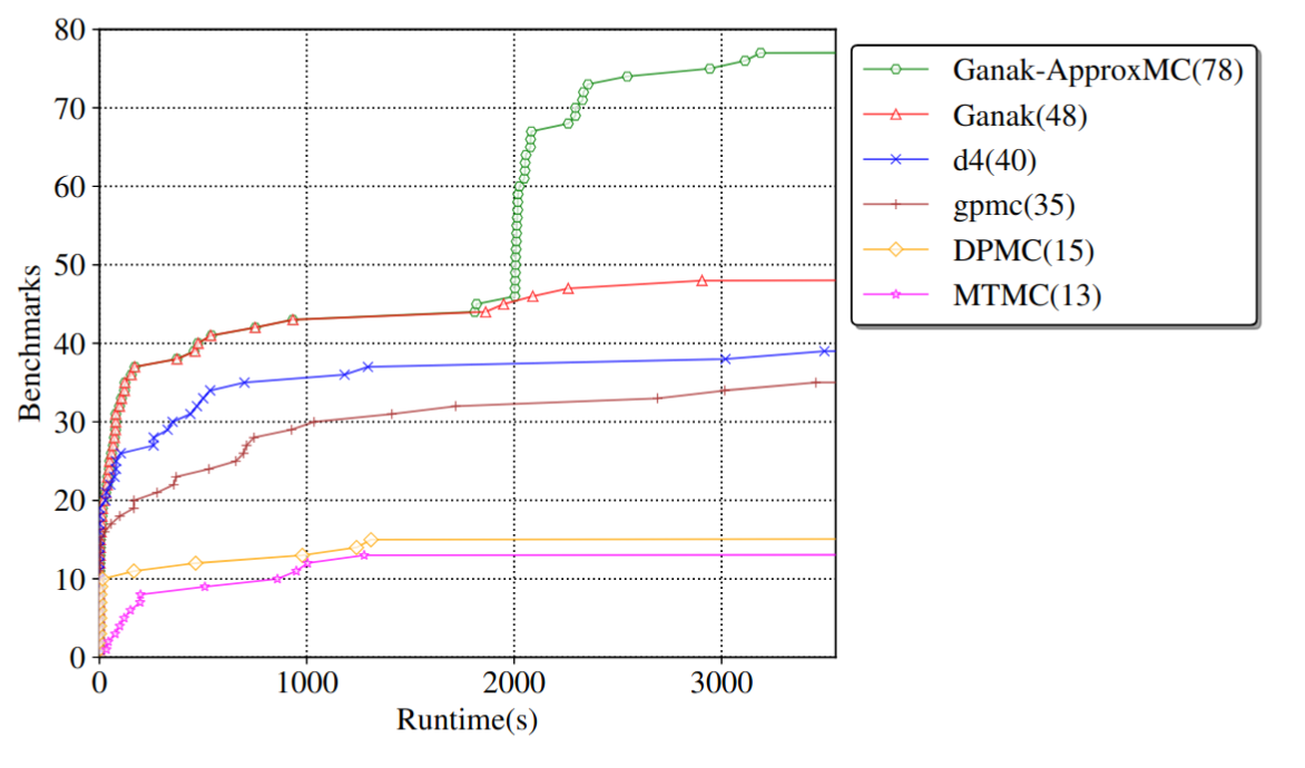
How Approximate Model Counting Works

Approximate model counting allows to count the number of solutions (or “models”) to propositional satisfiability problems. This problem seems trivial at first given a propositional solver that can find a single solution: find one solution, ban it, ask for another one, ban it, etc. until all solutions are counted. The issue is that sometimes, the number of solutions is 2^50 and so counting this way is too slow. There are about 2^266 atoms in the universe, so counting anywhere near that is impossible using this method.

Exact Counting

Since we cannot count 1-by-1, we are then left with trying to count in some smarter way. There are a bunch of methods to count exactly, the simplest is to cut the problem on a variable, count when the variable is True, count when the variable is False, recursively, and add them all up. Given caching of components that recur while “cutting” away, this can be quite successful, as implemented by sharpSAT (see Marc Thurley’s paper).

These counters can scale quite well, but have some downsides. In particular, when the memory runs out, the cache needs to be groomed, sometimes resorting back to 1-by-1 counting, which we know will fail as there is no way 2^200 can be counted 1-by-1 in any reasonable amount of time. The caching systems used are smart, though, retaining last-used entries when the cache needs to be groomed. However, sometimes this grooming algorithm can lead to cyclic behaviour that effectively simulates 1-by-1 counting.

Approximate Counting

What Chakraborty, Meel and Vardi did in their paper, was to create a counter that counts not exactly, but “probably approximately correctly”. This jumble of terms basically means: there is a certain probability that the counting is correct, within a given threshold. We can both improve the probability and the threshold given more CPU time spent. In practical terms, the probability can be set to be over 99.99% and the threshold can be set to be under 20%, still beating exact counters. Note that 20% is not so much, as e.g. 2^60*1.2 = 2^(60.3).

A Galton Box

So what’s the trick? How can we approximately count and give guarantees about the count? The trick is in fact quite simple. Let’s say you have to count balls, and there are thousands of them. One way to do it is to count 1-by-1. But, if you have a machine that can approximately half the number of balls you have, it can be done a lot faster: you half the balls, then check if you have at least 5 doing 1-by-1 counting. If you do, you half them again, and check if you have at least 5, etc. Eventually, let’s say you halved it 11 times and now you are left with 3 balls. So approximately, you must have had 3*2^11 = 6144 balls to begin with. In the end you had to execute the 1-by-1 count only 11*5+3+1 =59 times — a lot less than 6144! This is the idea used by ApproxMC.

Approximately Halving Using XORs

The “approximate halving” function used by ApproxMC is the plain XOR function, populated with variables picked with 50% probability. So for example if we have variables v1…v10, we pick each variable with 50% probability and add them into the same XOR. Let’s say we picked v1,v2,v5 and v8. The XOR would then be: v1⊕v2⊕v5⊕v8=1. This XOR is satisfied if an odd number of variables from the set {v1,v2,v5,v8} are 1. This intuitively forbids about half the solutions. The “intuitively” part of course is not enough, and if you read the original paper you will find the rigorous mathematical proof for the approximate halving of solutions this XOR function provides.

OK, so all we need to do is add these XORs to our original problem and we are done! This sounds easy, but there is a small hurdle and there is a big hurdle associated with this.

The small hurdle is that the original problem is a CNF, i.e. a conjunction of disjunctions, looking like “(v1 OR v2) AND (v2 OR not v3 OR not v4) AND…”. The XOR obviously does not look like this. The straightforward translation of XOR into CNF is exponential, so we need to add some variables to cut them smaller. It’s not that hard to figure this out and eventually add all the XORs into the CNF.

XORs, CDCL, and Gauss-Jordan Elimination

The larger hurdle is that once the XORs are in the CNF using the translation, the CNF becomes exponentially hard to solve using standard CDCL as used in most SAT solvers. This is because Gauss-Jordan elimination is exponentially hard for the standard CDCL to perform — but we need Gauss-Jordan elimination because the XORs will interact with each other, as we expect there to be many of them. Without being able to resolve the XORs with each other efficiently and derive information from them, it will be practically impossible to solve the CNF.

The solution is to tightly integrate Gauss-Jordan elimination into the solving process. CryptoMiniSat was the first solver to do this tight integration (albeit only for Gaussian elimination, which is sufficient). Other solvers have followed, in particular the work by Tero Laitinen and work by Cheng-Shen Han and Jie-Hong Roland Jiang. CryptoMiniSat currently uses the code by Han and Jiang after some cleanup and updates.

The latest work on ApproxMC and CryptoMiniSat has added one more thing besides the tight integration of the CDCL cycle: it now allows in- and pre-processing to occur while the XORs are inside the system. This brought some serious speedups as pre- and inprocessing are important factors in SAT solving. In fact, all modern SAT solvers strongly depend on them being active and working.

Concluding Remarks

We have gone from what model counting is, through how approximate counting works from a high-level perspective, all the way to the detail of running such a system inside a modern SAT solver. In case you want to try it out, you can do it by downloading the pre-built binaries or building it from source.