Uniform sampling is a problem where you are given a solution space and you have to present solutions uniformly, at random. In some cases, this is quite simple, say, for the lotto. Just pick 5 random numbers from a box and we are done! For the lotto the solution space is very easy to generate. However, when there are constraints on the solution space, it starts to get tricky.
Let’s say that I have a function I want to test, but the input to the function has some real-world constraints like e.g. the 1st parameter must be larger than the second, the 2nd parameter must be divisible by the 3rd etc. If I want to test that this function operates correctly, one way to do it is to generate 100 uniformly random inputs that don’t violate any of the constraints, run the function, and see if all is OK. For this, I need a fast way of generating uniform samples given the constraints on the solution space.
Sampler speed vs. accuracy
There have been many samplers proposed in the literature. I personally have worked on one called UniGen, a guaranteed approximate probabilistic sampler, meaning that it’ll give approximately uniform samples most of the time, and we have a proof to back this up. It’s a great sampler and will work very fast on many instances. However, for really complex solution spaces, it can have trouble. Say, you want to generate interesting test inputs for your deep learning algorithm. Deep neural networks tend to be extremely complex when translated to binary constraints, so UniGen will likely not be fast enough. It would give very good quality samples (i.e. properly uniform samples), but if it’s too slow, we may want to exchange quality of samples for speed of generation.
There are two well-known samplers that are supposed to generate uniform samples on complex solution spaces, QuickSampler (code), and STS (code), but give no guarantees, let’s call these “uniform-like” samplers. Unfortunately, the paper by Chakraborty et al and its resulting code Barbarik showed that these uniform-like samplers are highly non-uniform. Barbarik is a pretty neat idea that basically constructs solution spaces with known solution distributions and then asks the sampler to generate uniform samples. Knowing the solution space, Barbarik can then verify how non-uniform the sampler is. Imagine having a box with 1000 balls, half of them blue and the other half green. Now if I ask the sampler to give me 50 balls at random, and all of them are green, I’d be a bit surprised to say the least. It’d be like the 5-lottery having the same numbers 3 times in a row. Possible, but… not very likely. If I do this experiment 100 times, and I always get 50 green balls, it’s fair to conclude that the sampler is not uniform.
Our new uniform-like sampler, CMSGen
Given an effective tester, Barbarik, we (Priyanka Golia, Sourav Chakraborty, Kuldeep S. Meel, and myself) thought perhaps we can follow the nowadays very successful test-driven development (TDD) methodology. All we have to do is to make our sampler pass the test of Barbarik, while being at least as fast as STS/QuickSampler, and we’ll be good to go. In fact, given Barbarik, it only took about a week of playing around with CryptoMiniSat’s options to beat both STS and QuickSampler in both accuracy and speed. This speaks volumes to how important it is to have a robust, reliable, and fast testing framework that can give immediate feedback about the quality of samples generated.
Our new uniform-like sampler, based on CryptoMiniSat, is called CMSGen (research paper here), and effectively takes CyrptoMiniSat and applies the following set of changes, through pre-set command line options:
- Pick polarities at random. Normally, SAT solvers use polarity caching scheme, but of course we want uniform samples over all the search space, so we need to pick polarities at random.
- Branch on variables at random. Normally, SAT solver branch on variables that will most likely lead to a conflict to maximize search efficiency (the VSIDS heuristic). However, we want to explore the solution space as evenly as possible, and so we want to approach the solution space from as many angles as possible. If you think about the search space as an N-dimensional binary cube, then we are trying to approach this cube as any ways as possible.
- Turn off all pre- and inprocessing. Pre and inprocessing in SAT solvers are used to minimize the instance, transforming it into something easier to solve, e.g. through Bounded Variable Elimination. We later reconstruct a viable solution based on the solution to the transformed instance. However, the transformed instance may (and often will!) have a very different solution space. We cannot have that, so we must turn this off. To be fair, some pre- and inprocessing could be left intact, e.g. subsumption and self-subsuming elimination, perhaps a future paper :)
- Restart at static intervals. Restarts are nowadays often dynamic in modern SAT solvers, or even if not dynamic, then follow a non-regular pattern. However, that could disturb how we find solution. Imagine, let’s say that solutions with variable A set to TRUE are very easy to find, but solutions with FALSE are very hard to find. What will happen? Well, in restarts where A was randomly set to TRUE, we’ll always quickly find a solution and output it. But for restarts when A was randomly set to FALSE, the system would struggle to find a solution, and after some conflicts, it will simply restart into a status where hopefully A is set to TRUE, and it can find a solution again. It is quite clear to see that this will lead to serious issues with sampling quality. Hence, we set an adjustable but static restart interval of 100 conflicts, with higher values typically leading to more uniform samples.
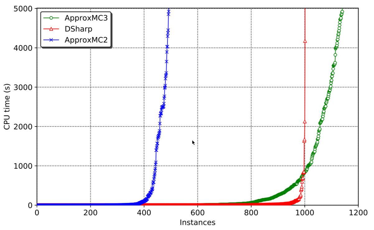
Performance of CMSGen
Performance of the system is on the ridiculous scale in comparison with other samplers:
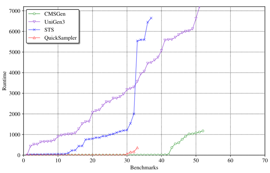
When it comes to 2-wise coverage, i.e. the quality of samples, the data speaks for itself (note, UniGen is missing here because it was too slow):
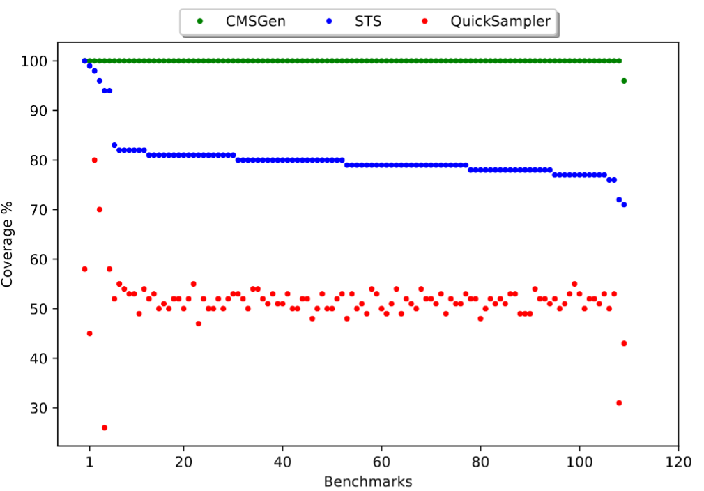
Note that between STS and QuickSampler, STS is both the more uniform sampler, but also the slower one. CMSGen overcomes this limitation: it’s both faster than QuickSampler, and more uniform than STS.
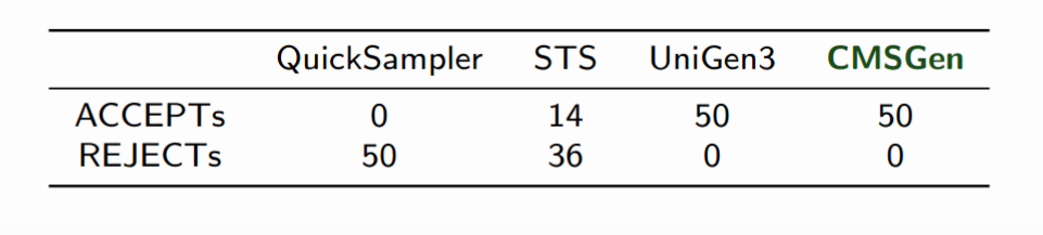
And of course, the Barbarik tester gives “Accept” on CMSGen much more often than on STS or QuickSampler:
Conclusion
If you need non-guaranteed uniform but fast sampling, I’d go and try out CMSGen. It’s really a completely different beast. It’s not a guaranteed uniform sampler, but it’s incredibly effective. In fact, it’s so effective and works so well, it took me a full year to figure out how best to generate problems for it where it wouldn’t be uniform. But that’s another paper, and another blog post! In the meantime, the sampler is here, go check it out!