Tag Archives: Gaussian elimination

How Approximate Model Counting Works

Approximate model counting allows to count the number of solutions (or “models”) to propositional satisfiability problems. This problem seems trivial at first given a propositional solver that can find a single solution: find one solution, ban it, ask for another one, ban it, etc. until all solutions are counted. The issue is that sometimes, the number of solutions is 2^50 and so counting this way is too slow. There are about 2^266 atoms in the universe, so counting anywhere near that is impossible using this method.

Exact Counting

Since we cannot count 1-by-1, we are then left with trying to count in some smarter way. There are a bunch of methods to count exactly, the simplest is to cut the problem on a variable, count when the variable is True, count when the variable is False, recursively, and add them all up. Given caching of components that recur while “cutting” away, this can be quite successful, as implemented by sharpSAT (see Marc Thurley’s paper).

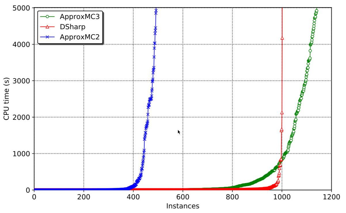
These counters can scale quite well, but have some downsides. In particular, when the memory runs out, the cache needs to be groomed, sometimes resorting back to 1-by-1 counting, which we know will fail as there is no way 2^200 can be counted 1-by-1 in any reasonable amount of time. The caching systems used are smart, though, retaining last-used entries when the cache needs to be groomed. However, sometimes this grooming algorithm can lead to cyclic behaviour that effectively simulates 1-by-1 counting.

Approximate Counting

What Chakraborty, Meel and Vardi did in their paper, was to create a counter that counts not exactly, but “probably approximately correctly”. This jumble of terms basically means: there is a certain probability that the counting is correct, within a given threshold. We can both improve the probability and the threshold given more CPU time spent. In practical terms, the probability can be set to be over 99.99% and the threshold can be set to be under 20%, still beating exact counters. Note that 20% is not so much, as e.g. 2^60*1.2 = 2^(60.3).

A Galton Box

So what’s the trick? How can we approximately count and give guarantees about the count? The trick is in fact quite simple. Let’s say you have to count balls, and there are thousands of them. One way to do it is to count 1-by-1. But, if you have a machine that can approximately half the number of balls you have, it can be done a lot faster: you half the balls, then check if you have at least 5 doing 1-by-1 counting. If you do, you half them again, and check if you have at least 5, etc. Eventually, let’s say you halved it 11 times and now you are left with 3 balls. So approximately, you must have had 3*2^11 = 6144 balls to begin with. In the end you had to execute the 1-by-1 count only 11*5+3+1 =59 times — a lot less than 6144! This is the idea used by ApproxMC.

Approximately Halving Using XORs

The “approximate halving” function used by ApproxMC is the plain XOR function, populated with variables picked with 50% probability. So for example if we have variables v1…v10, we pick each variable with 50% probability and add them into the same XOR. Let’s say we picked v1,v2,v5 and v8. The XOR would then be: v1⊕v2⊕v5⊕v8=1. This XOR is satisfied if an odd number of variables from the set {v1,v2,v5,v8} are 1. This intuitively forbids about half the solutions. The “intuitively” part of course is not enough, and if you read the original paper you will find the rigorous mathematical proof for the approximate halving of solutions this XOR function provides.

OK, so all we need to do is add these XORs to our original problem and we are done! This sounds easy, but there is a small hurdle and there is a big hurdle associated with this.

The small hurdle is that the original problem is a CNF, i.e. a conjunction of disjunctions, looking like “(v1 OR v2) AND (v2 OR not v3 OR not v4) AND…”. The XOR obviously does not look like this. The straightforward translation of XOR into CNF is exponential, so we need to add some variables to cut them smaller. It’s not that hard to figure this out and eventually add all the XORs into the CNF.

XORs, CDCL, and Gauss-Jordan Elimination

The larger hurdle is that once the XORs are in the CNF using the translation, the CNF becomes exponentially hard to solve using standard CDCL as used in most SAT solvers. This is because Gauss-Jordan elimination is exponentially hard for the standard CDCL to perform — but we need Gauss-Jordan elimination because the XORs will interact with each other, as we expect there to be many of them. Without being able to resolve the XORs with each other efficiently and derive information from them, it will be practically impossible to solve the CNF.

The solution is to tightly integrate Gauss-Jordan elimination into the solving process. CryptoMiniSat was the first solver to do this tight integration (albeit only for Gaussian elimination, which is sufficient). Other solvers have followed, in particular the work by Tero Laitinen and work by Cheng-Shen Han and Jie-Hong Roland Jiang. CryptoMiniSat currently uses the code by Han and Jiang after some cleanup and updates.

The latest work on ApproxMC and CryptoMiniSat has added one more thing besides the tight integration of the CDCL cycle: it now allows in- and pre-processing to occur while the XORs are inside the system. This brought some serious speedups as pre- and inprocessing are important factors in SAT solving. In fact, all modern SAT solvers strongly depend on them being active and working.

Concluding Remarks

We have gone from what model counting is, through how approximate counting works from a high-level perspective, all the way to the detail of running such a system inside a modern SAT solver. In case you want to try it out, you can do it by downloading the pre-built binaries or building it from source.

ApproxMCv3, a modern approximate model counter

This blogpost and its underlying work has been brewing for many years, and I’m extremely happy to be able to share it with you now. Kuldeep Meel and myself have been working very hard on speeding up approximate model counting for SAT and I think we have made real progress. The research paper, accepted at AAAI-19 is available here. The code is available here (release with static binary here). The main result is that we can solve a lot more problems than before. The speed of solving is orders(!) of magnitude faster than the previous best system:

Background

The idea of approximate model counting, originally by Chakraborty, Meel and Vardi was a huge hit back in 2013, and many papers have followed it, trying to improve its results. All of them were basically tied to CryptoMiniSat, the SAT solver that I maintain, as all of them relied on XOR constraints being added to the regular CNF of a typical SAT problem.

So it made sense to examine what CryptoMiniSat could do to improve the speed of approximate counting. This time interestingly coincided with me giving up on XORs in CryptoMiniSat. The problem was the following. A lot of new in- and preprocessing systems were being invented, mostly by Armin Biere et al, and I quickly realised that I simply couldn’t keep adding them, because they didn’t take into account XOR constraints. They handled CNF just fine, but not XORs. So XORs became a burden, and I removed them in versions 3 and 4 of CryptoMiniSat. But there was need, and Kuldeep made it very clear to me that this is an exciting area. So, they had to come back.

Blast-Inprocess-Recover-Destroy

But how to both have and not have XOR constraints? Re-inventing all the algorithms for XORs was not a viable option. The solution I came up with was a rather trivial one: forget the XORs during inprocessing and recover them after. The CNF would always remain the source of truth. Extracting all the XORs after in- and preprocessing would allow me to run the Gauss-Jordan elimination on the XORs post-recovery. So I can have the cake and eat it too.

The process is conceptually quite easy:

  1. Blast all XORs into clauses that are in the input using intermediate variables. I had all the setup for this, as I was doing Bounded Variable Addition  (also by Biere et al.) so I didn’t have to write code to “hide” these additional variables.
  2. Perform pre- or inprocessing. I actually only do inprocessing nowadays (as it has faster startup time). But preprocessing is just inprocessing at the start ;)
  3. Recover the XORs from the CNF. There were some trivial methods around. They didn’t work as well as one would have hoped, but more on that later
  4. Run the CDCL and Gauss-Jordan code at the same time.
  5. Destroy the XORs and goto 2.

This system allows for everything to be in CNF form, lifting the XORs out when necessary and then forgetting them when it’s convenient. All of these steps are rather trivial, except, as I later found out, recovery.

XOR recovery

Recovering XORs sounds like a trivial task. Let’s say we have the following clauses

 x1 V  x2 V  x3
-x1 V -x2 V  x3
 x1 V -x2 V -x3
-x1 V  x2 V -x3

This is conceptually equivalent to the XOR v1+v2+v3=1. So recovering this is trivial, and has been done before, by Heule in particular, in his PhD thesis. The issue with the above is the following: a stronger system than the above still implies the XOR, but doesn’t look the same. Let me give an example:

 x1 V  x2 V  x3
-x1 V -x2 V  x3
 x1 V -x2 V -x3
-x1 V  x2

This is almost equivalent to the previous set of clauses, but misses a literal from one of the clauses. It still implies the XOR of course. Now what? And what to do when missing literals mean that an entire clause can be missing? The algorithm to recover XORs in such cases is non-trivial. It’s non-trivial not only because of the complexity of how many combinations of missing literals and clauses there can be (it’s exponential) but because one must do this work extremely fast because SAT solvers are sensitive to time.

The algorithm that is in the paper explains all the bit-fiddling and cache-friendly data layout used along with some fun algorithms that I’m sure some people will like. We even managed to use compiler intrinsics to use target-specific assembly instructions for hamming weight calculation. It’s a blast. Take a look.

The results

The results, as shown above, speak for themselves. Problems that took thousands of seconds to solve can now be solved under 20. The reason for such incredible speedup is basically the following. CryptoMiniSatv2 was way too clunky and didn’t have all the fun stuff that CryptoMiniSatv5 has, plus the XOR handling was incorrect, loosing XORs and the like. The published algorithm solves the underlying issue and allows CNF pre- and inprocessing to happen independent of XORs, thus enabling CryptoMiniSatv5 to be used in all its glory. And CryptoMiniSatv5 is fast, as per the this year’s SAT Competition results.

Some closing words

Finally, I want to say thank you to Kuldeep Meel who got me into the National University of Singapore to do the work above and lots of other cool work, that we will hopefully publish soon. I would also like to thank the National Supercomputing Center Singapore  that allowed us to run a ton of benchmarks on their machines, using at least 200 thousand CPU hours to make this paper. This gave us the chance to debug all the weird edge-cases and get this system up to speed where it beats the best exact counters by a wide margin. Finally, thanks to all the great people I had the chance to meet and sometimes work with at NUS, it was a really nice time.

Why CryptoMiniSat 3.3 doesn’t have XORs

I’ve had a number of inquiries about why CryptoMiniSat 3.3 doesn’t have native XOR clause support. Let me explain what I think the benefits and the drawbacks are of having native XOR support and why I made the choice of removing them.

Benefits

The most trivial benefit is that users don’t have to translate XORs into plain CNF. Although transforming is rather easy, some prefer not to go through the hassle. The principle is to cut the XOR into smaller XORs by introducing new variables and then representing the cut-down XORs by banning all the wrong combinations. For example the the XOR x+y+z+w=0 is cut into two XORs x+y+r=0, z+w+r=0 and then x+y+r=0 is represented as x \vee y \vee r, x \vee \neg y \vee \neg r, \ldots.

A more substantial benefit is that propagation and conflict generation can be done natively. This is quite advantageous as it means that far less clauses and variables need to be visited while propagating and generating the UIP conflict. Less variables and clauses visited means less cache-misses and due to the more compact representation, less memory overhead and thus even better cache usage. (For the aficionados: an interesting side-effect of XORs is that blocked literals cannot be used for XOR clauses).

The biggest benefit of having native XORs is that Gaussian elimination can be carried out at every level of the search tree, not just at top-level. Although most people I have talked with still think that CryptoMiniSat 2 only performs Gaussian elimination only at top-level, this is not the case. Performing Gauss at top-level is a two-day hack. Performing it at every level took me about half a year to implement (and about 5K lines of code). It requires leaving traces of past computations and computing reasons for propagations and conflicts indicated by the Gaussian elimination algorithm. According to my highly unofficial count, exactly 2 people use Gaussian elimination at deeper than top-level, Vegard Nossum and Kuldeep S Meel. Out of these two users, only the latter have indicated speedups. It speeds up crypto problems, but not many others, so it’s completely disabled by default.

Drawbacks

The main drawback of having native XOR clauses along normal CNF clauses is the loss of simplicity and universality. Let me explain in detail.

Loss of simplicity. Once a variable present in both a normal and an XOR clause, it cannot be eliminated in a simple way. I don’t even want to try to express the clauses that would result from doing varelim in such cases — it’s probably horribly convoluted. All algorithms in the code now need to check for XORs. On-the-fly clause strengthening cannot strengthen an XOR with a normal clause, of course. Clause cleaning has to take into account that when a 3-long XOR is shortened to a 2-long one, it indicates a new equivalent literal and that may lead to immediate UNSAT. I could go on, but the list is long.

Another problem is that XORs make the state more complex. Until now there were only clauses of the form a \vee \neg b \ldots, sometimes specially stored such as binary clauses. The state of the solver goes through many transformations — think of them as llvm passes — while it is in-processed and solved. The more complex the state, the larger and the more complex the code. While a simple clause-cleaning algorithm can be expressed in about 20 lines of code without implicit binary&tertiary clauses, the same algo blows up to about 100 lines of code with those optimizations. Once you add XOR clauses, it jumps to around double that. We just made our code 10x larger. Imagine adding native support for, e.g. at-most-n.

Loss of universality. If a variable is only XOR clauses, it can now be eliminated at the XOR level. A pure variable at the XOR level indicates an XOR clause that can be removed and later always satisfied. XOR subsumption is when an XOR subsumes the other: the larger can be removed and their XOR added in. All of these are implemented in CMS 2. Probably there are many others out there, though. We could try to implement them all, but this is a whole new universe that may open up the gates of hell. Worst of all, most of these techniques on XORs are probably already simulated by in-processing techniques at the CNF level. Pure XOR variables are simulated by blocked clause elimination. XOR-based variable elimination doesn’t make practical sense at the CNF level, but it could be simulated by normal variable elimination if ignoring heuristics. I could go on.

What CryptoMiniSat 3.3 does

The compromise I came up with for CryptoMiniSat 3.0 is that I regularly search for XOR clauses at the top-level, perform top-level Gaussian elimination, and add the resulting new information to the CNF. Binary and unitary XOR clauses are the simplest to add back.

In the SAT’11 application benchmark set, out of 300 problems, 256 problems contain XOR clauses. the number of XOR clauses found, when they are found, is on average 2905 with an average size of 4.2 literals. Using Gaussian elimination, counting only when something was extracted, the average number of literal equivalences (binary XORs) extracted is 130, while the number of unitary clauses extracted is 0.15.

Here is a typical example output:

c Reading file 'valves-gates-1-k617-unsat.shuffled-as.sat03-412.cnf.gz'
c -- header says num vars:         985042
c -- header says num clauses:     3113540
[.. after about 124K conflicts ..]
c XOR finding  Num XORs: 104091 avg size:  3.0 T: 2.11
c Cut XORs into 2185 block(s) sum vars: 180818 T: 0.11
c Extracted XOR info. Units: 0 Bins: 1275 0-depth-assigns: 0 T: 8.34

Here, about 104K XOR clauses were found (using a sophisticated algorithm) within 2.11s, all of size 3. These XOR clauses were subjected to disconnected component analysis (within the XOR sphere) and they were found to belong to 2185 components. It is important to cut XORs into groups, because Gaussian elimination is an O(n^{\approx 2.5}) algorithm and if we can reduce the n by having more than one matrix, the speed is significantly increased. Next, these 2185 matrices were Gauss-eliminated and were found to contain 1275 binary XOR clauses, which were quickly marked as equivalent literals.

To perform Gaussian elimination at top-level, CryptoMiniSat uses the excellent m4ri library, maintained by my old college and friend Martin Albrecht. It’s a lightweight yet extremely fast Gaussian elimination system using all sorts of nifty tricks to do its job. Unfortunately, for large matrices it can still take a long while as the algorithm itself is not cheap, so I have a cut-off for matrices that are too large.

What a future CryptoMiniSat 3.x could do

Once we have extracted the XORs, we could just as well keep them around during search and perform Gaussian elimination at levels below the top-level. This would bring us close to the old system in terms of real performance — native propagation (which would be unavailable) can only give a 1.5x-2x speedup, but Gaussian elimination at every level can give much more. I would need to clean up a lot of code and then, maybe, this would work. Maybe I’ll do this one day. Though, after spending weeks doing it, probably people will still believe it only does top-level. At least right now, it’s the case.

Conclusions

Implementing a new theory such as XOR deep into the guts of a SAT solver is neither easy nor does it provide a clear advantage in most situations. Those who push for these native theories have either not tried implementing them into a complicated solver such as lingeling/SatELite/CryptoMiniSat/clasp or have already bit the bullet such as the clasp group and I did, and it is probably limiting them in extending the system with new techniques. The resulting larger internal state leads to edge cases, exceptions, and much-much more code.

Gaussian elimination is released

The new CryptoMiniSat, version 2.4.2 now has on-the-fly Gaussian elimination compiled in by default. You can simply use it by issuing e.g.

./cryptominisat --gaussuntil=100 trivium-cipher.cnf

and enjoy outputs such as:

c gauss unit truths : 0
c gauss called : 31323
c gauss conflicts : 5893 (18.81 %)
c gauss propagations : 7823 (24.98 %)
c gauss useful : 43.79 %
c conflicts : 34186 (4073.39 / sec)
c decisions : 39715 (6.86 % random)

Which basically tells that gaussian elimination was called 31 thousand times out of 39 thousand, and so it was essentially running almost all the time. Out of the 31’323 times it was called, 44% of the cases it found either a conflict or a propagation. This is a very good result, and is typical of the Trivium cipher. Trivium can be speeded up by up to 2x with Gaussian elimination. I will put up lots of CNFs, so you will be able to play around with them and (optionally) verify these results.

The magic parameter “–gaussuntil=100” tells the program to execute Gaussian elimination until decision level 100, and no deeper. I haven’t implemented and automation into finding the best depth, and so I use this (very) crude fixed number 100. Probably better results could be achieved with a fine tuning of the depth cut-off, but I don’t have the time for the moment to play around with it. However, if you are interested, you will be able to try out different depths, different ciphers, etc. I will shortly be releasing a tool called “Grain of Salt” to generate CNFs for any shift-register based stream cipher, so you can test them against CryptoMiniSat or any other SAT solver.

I hope you will enjoy using on-the-fly Gaussian elimination in CryptoMiniSat 2.4.2!