After many years of work, I am very happy to present our new CNF model counting preprocessor, Arjun [PDF][static binary]. It improves upon our approximate model counter ApproxMC [static binary], and can be used as a stand-alone binary to preprocess CNFs for (projected) model counting . Usage is simple:
./arjun blasted_case110.cnf
c Arjun Version: 43b17ef5899c461b8e947b0f3ca286efcf71464c
c CMS SHA revision 9bf1d82a7b9fa5492cf4f0437cf7110b77ad7230
[..]
c [arjun] original sampling set size: 284
c [arjun] final set size:   15 percent of original: 5.2817 %
Here, Arjun took a CNF that had a projection set of 284 variables, and reduced it to an independent support of only 15 variables. Arjun is now part of ApproxMC by default. Let’s solve a problem with ApproxMC without Arjun:
./approxmc --arjun 0 blasted_squaring42.cnf.gz.no_w.cnf.gz
c ApproxMC SHA revision 9fb4fdd01b40cc0526c4933e2f2dca402f0ab91f
c CMS SHA revision 9bf1d82a7b9fa5492cf4f0437cf7110b77ad7230
c [appmc] Orig sampling vars size: 349
[after waiting 5000 seconds, it times out]
Now let’s do the same with Arjun (this does not use code from SharpSAT-td):
./approxmc blasted_squaring42.cnf.gz.no_w.cnf.gz
c ApproxMC SHA revision 9fb4fdd01b40cc0526c4933e2f2dca402f0ab91f
c CMS SHA revision 9bf1d82a7b9fa5492cf4f0437cf7110b77ad7230
c Arjun SHA revision 43b17ef5899c461b8e947b0f3ca286efcf71464c
c [appmc] Orig sampling vars size: 349
c [arjun] final set size:  155 percent of original: 44.4126 %
c [appmc+arjun] Total time: 12.80
c [appmc] Number of solutions is: 80*2**127
s SATISFIABLE
s mc 13611294676837538538534984297270728458240
Done in 12.8 seconds, NICE. Wanna try it out? Arjun+ApproxMC static Linux binary HERE, Arjun static Linux binary HERE. Research paper HERE. Arjun code HERE. Now that the demo is out of the way, let’s get into the nitty-gritty details!
Projected Model Counting
CNF model counting is the problem where you want to count the number of solutions to a set of equations written in the CNF form. This form is quite restrictive, but also very powerful, here is an example:
 x1 OR  x2 OR -x3 = True
 x1 OR -x2 = True
 x1 OR -x3 = True
 x1 OR -x4 = True
-x1 OR  x4 = True
The above set of constraints clearly have a solution, e.g. setting x1=True and x4=False will satisfy all constraints. The question in model counting is how many solutions a system has. The above problem has 5 solutions in total:
[Where "1" means TRUE and "-1" means FALSE]
x1   x2  x3  x4
-----------------
-1  -2  -3   4 0
 1   2   3  -4 0
 1   2  -3  -4 0
 1  -2   3  -4 0
 1  -2  -3  -4 0
This was kinda easy. However, there are two complications. One complication tends to be is that there are a massive number of solutions. For example, there are 2^200 solutions. Enumerating them one-by-one is just not going to work. Hence, we need some smart systems to do the counting for us, that don’t count one-by-one. Secondly, often we are interested only in the distinct number of solutions over a certain set of variables. Let’s take the above example, and say we want the distinct number of solutions over variables x1, x2 and x4 only. So, let’s delete column for x3 from above table:
x1   x2  x4   Same?
-------------------
-1  -2   4 0
 1   2  -4 0  *
 1   2  -4 0  *
 1  -2  -4 0  +
 1  -2  -4 0  +
Notice there are only 3 distinct solutions: the rows marked with * are both the same, and the rows marked with + are also the same. This is called projected counting because we are projecting the solution space over a specific set of variables — in this case, x1, x2, and x4.
Computing the Independent set of a Projection Set
In the above example, our projection set was x1, x2, and x4. However, notice that x1=-x4, due to the constraints:
 x1 OR -x4 = True
-x1 OR  x4 = True
Hence, it is good enough to count over x1 and x2, since x4 is determined by x1 and so x4 cannot possibly make the distinct number of solutions smaller or larger. This realization is at the heart of calculating an independent support — we basically want to minimize the set of variables that we project over. The independent support is simply a subset of the projection set, that’s hopefully a lot smaller than the projection set.
An early work on independent support calculation is the B+E preprocessor [PDF], which aims to do two things: “B” which finds a small independent support, and “E”, which eliminates variables from the problem. Let’s concentrate on “B” here. In the B+E paper, the authors talk about independent support over all variables of the formula, not over a projection set. In other words, their code and paper originally was conceived to minimize a projection set that had all variables inside. In our case, their work would minimize x1..x4, finding that x1,x2,x3 is an independent support of x1..x4.
Implicit Definability
The trick of B+E is to use the idea of so-called implicit definability. Implicit deniability is really simple. If I take x1, x2 and x3, does that define the value of x4? Yep. In fact, x1 on its own would define the value of x4, because x1=-x4. However, sometimes you have equations that define a variable through a (large) number of other variables. For example:
 x30 OR -x10 OR -x20 = True
-x30 OR  x10 = True
-x30 OR  x20 = True
This set of constraints describe x10 AND x20=x30. In this case, x10 and x20 together define x30. So if you have the above set of constraints in a CNF, and you have x10, x20, and x30 all in your projection set, you can confidently take out x30 from the set — and the number of distinct solutions projected will not change.
Implicit definability states that we can find these definitions in an implicit way, using a relatively straightforward system. We make two copies of the CNF, let’s call these CNF1 and CNF2. Then, we have variables v1…vN in the first CNF and w1..wN in the second CNF. Now, we create new variables called indicator variables, i1…iN that indicate whether v1=w1, v2=w2… etc. After this setup, the query is simple. Given i1=TRUE (i.e. given v1=w2), is it possible that v2 is different from w2? If it is, then our new independent set must contain both i1 and i2 (If not, we can get rid of i2). Now we move to i3. Let’s set i1=TRUE and i2=TRUE, and ask if it is possible that v3 is different from w3? Otherwise, our independent set remains i1, and we ask, is it possible that i1=TRUE and i2=TRUE, but v3 is different from w3? etc. This way, we test all the variables from v/w1…v/wN, and eventually end up with a set of indicator variables that tell us a minimal independent support.
Explicit Definability
As an external observer, without knowing nothing about implicit definability, CNF copying and renumbering and the like, it is quite easy to figure out that x1=-x4 just by looking at the CNF, since it contains:
 x1 OR -x4 = True
-x1 OR  x4 = True
Such set of constraints can be trivially found using Tarjan’s algorithm. This is actually linear in the number of binary (i.e. 2-long) constraints, so this is super-quick to run. Similarly, we can very easily find the AND gate x10 AND x20=x30:
 x30 OR -x10 OR -x20 = True
-x30 OR x10 = True
-x30 OR x20 = True
It’s a quick check on all the constraints that are 3-long and have the corresponding 2-long constraints. Such syntactic checks are well-known parts of SAT solvers. For example, the extremely successful kissat solver has the following lines of code in gates.c:
if (kissat_find_equivalence_gate (solver, lit))
  res = true;
else if (kissat_find_and_gate (solver, lit, 0))
  res = true;
else if (kissat_find_and_gate (solver, not_lit, 1))
  res = true;
else if (kissat_find_if_then_else_gate (solver, lit, 0))
  res = true;
else if (kissat_find_if_then_else_gate (solver, not_lit, 1))
  res = true;
else if (kissat_find_definition (solver, lit))
  res = true;
So, kissat finds equivalence gates (i.e. x1=x2), AND gates (like x10 AND x20=x30), IF-THEN-ELSE gates, and curiously… “definition” gates. What could these be? Well, it turns out kissat uses a very cool trick to find definitions. It takes all constraints that contain a variable, say x30/-x30, and cuts off the x30/-x30:
-x10 OR -x20 = True  <-- we cut of "x30 OR"
x10 = True           <-- we cut of "-x30 OR"
x20 = True           <-- we cut of "-x30 OR"
Notice that this set of constraints is now unsatisfiable. In fact, for all gates that define a variable, if you take all the constraints that the variable is in, and you chop off the variable, the constraints will together be unsatisfiable. To find such gates, kissat uses a SAT solver called kitten. Kitten solves these problems really fast and allows for UNSAT core extraction (not present in kissat) to find the defining variables.
Arjun
So what did we do with Arjun? We basically do the following set of improvements over B+E — while not even once looking at B+E’s code, since it was close-sourced, and by the time the authors open-sourced it, we already had our paper in the review queue:
- We allow taking in a projection set, rather than the full set of variables like B+E does. This allows us to compute and independent support of a projection set, which is extremely important for our model counter ApproxMC. With a small independent support, ApproxMC uses a smaller matrix, so Gauss-Jordan elimination, which is an O(n^3) algorithm in our implementation, is significantly faster.
- We use CryptoMiniSat to our advantage to simplify the CNF formula before running explicit or implicit definability detection. CryptoMiniSat is a powerful system that allows fine-tuned set of heuristics to be run, completely controlled from the API, e.g. “auto str = string(“intree-probe, occ-backw-sub-str, distill-bins, “); solver.simplify(NULL, &str);”
- We use all the different ways to syntactically recover gates: and/or gates, if-then-else gates, and parity (XOR) constraints. We also recover gates semi-syntactically using picosat (instead of kitten) — this is semi-syntactic, because we use syntactic methods to get the occurrence list of a variable and to construct the SAT query, but then use a SAT solver (i.e. a semantic method) to recover the definition, if any. We then construct a directed graph from the gates and greedily find a minimum cover. This is needed because there could be loops, and we don’t want x1 to be defined by x2, and x2 being defined by x1, and accidentally remove both, which would be silly.
- We repeat steps 2 & 3 at least 2x to make sure it’s done to a good enough level. This allows us to save time on the expensive next step, implicit definability detection. At this stage, we also do empty occurrence detection — if a variable is in the projection set, but doesn’t even occur in the formula, then obviously the variable can be removed and the count increased by a factor of 2.
- We change the SAT solver’s assumptions method to improve implicit definability detection. From the standpoint of a SAT solver, the queries mentioned in the implicit definability section are so-called assumption queries: assuming i1=TRUE, v2=TRUE, v3=FALSE, is there a solution? The list of assumptions tends to be very long here, so SAT solvers can struggle. Our insight here is to change the traditional way of how assumptions are handled in the SAT solver, and effectively make the SAT solver not backtrack to the beginning every time a query is made. This makes quite a bit of difference in performance.(Note: it turns out this improvement idea has been invented, and re-invented, a few times already, e.g. by SharpSAT-td, and by IntelSAT — see Alexander Nadel’s presentation at SAT 2022).
That’s all folks! These improvements add up to about 5k LoC of code. All in all, they make Arjun more than an order of magnitude faster than B+E, and it can compute an independent support over a projection set, rather than all variables in the formula.
Performance of Arjun
Here’s an example performance graph for B+E vs Arjun, using the set of benchmark instances we have been measuring the performance of ApproxMC on for ~5 years now — perhaps outdated, but at least it’s easy to compare all the values in all of our papers. The performance difference is quite big:
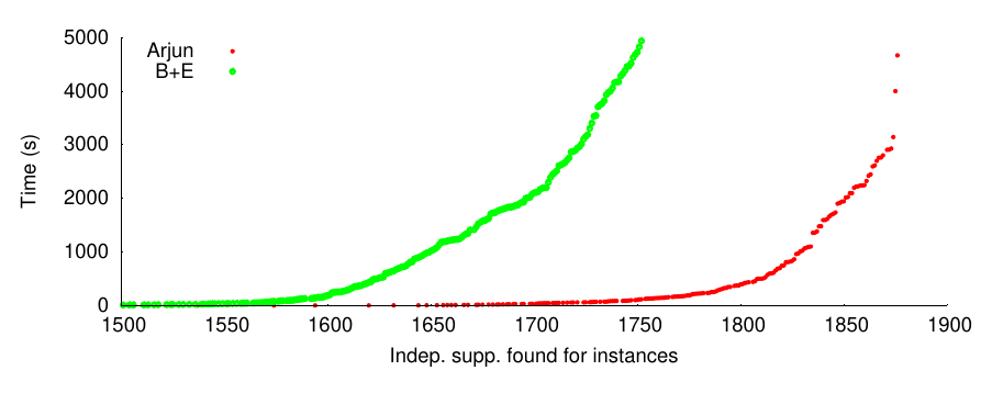
Basically, in B+E took 4932 seconds to compute the independent set of 1752 instances, while Arjun did the same in 117 seconds. Quite nice, about 40x improvement. Notice that due to the way our implicit definability works, it’s possible to e.g. order the variables in such a way as to make querying faster, but end up with a larger independent set. So, here is the comparison of independent sets computed by the same system as per the graph above:
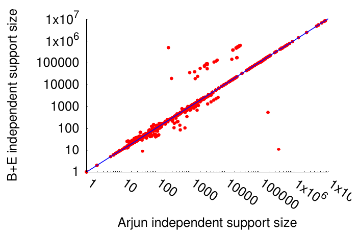
Essentially, the same, modulo some noise. There is some advantage to using B+E in a few cases, and there is some advantage using Arjun in other cases, from the perspective of the calculated independent set. However, notice that Arjun is so much faster, that we could actually run it 2x with different variable ordering, thereby getting a (much) smaller independent set, and often still be a lot faster than B+E. However, there is always a trade-off, so we decided to be approximately as good in the minimization as B+E, while being significantly faster.
Performance Impact on ApproxMC
So, Arjun is fast but what does that mean for ApproxMC? It turns out, it means a lot. ApproxMC adds XOR constraints over the projection set, and the smaller the projection set, the smaller the XORs . Hence, the matrix that the Gauss-Jordan elimination algorithm has to run on inside ApproxMC is much smaller — which is an O(n^3) algorithm in our implementation. Hence, the performance of ApproxMC4 vs Arjun+ApproxMC4 is remarkable:
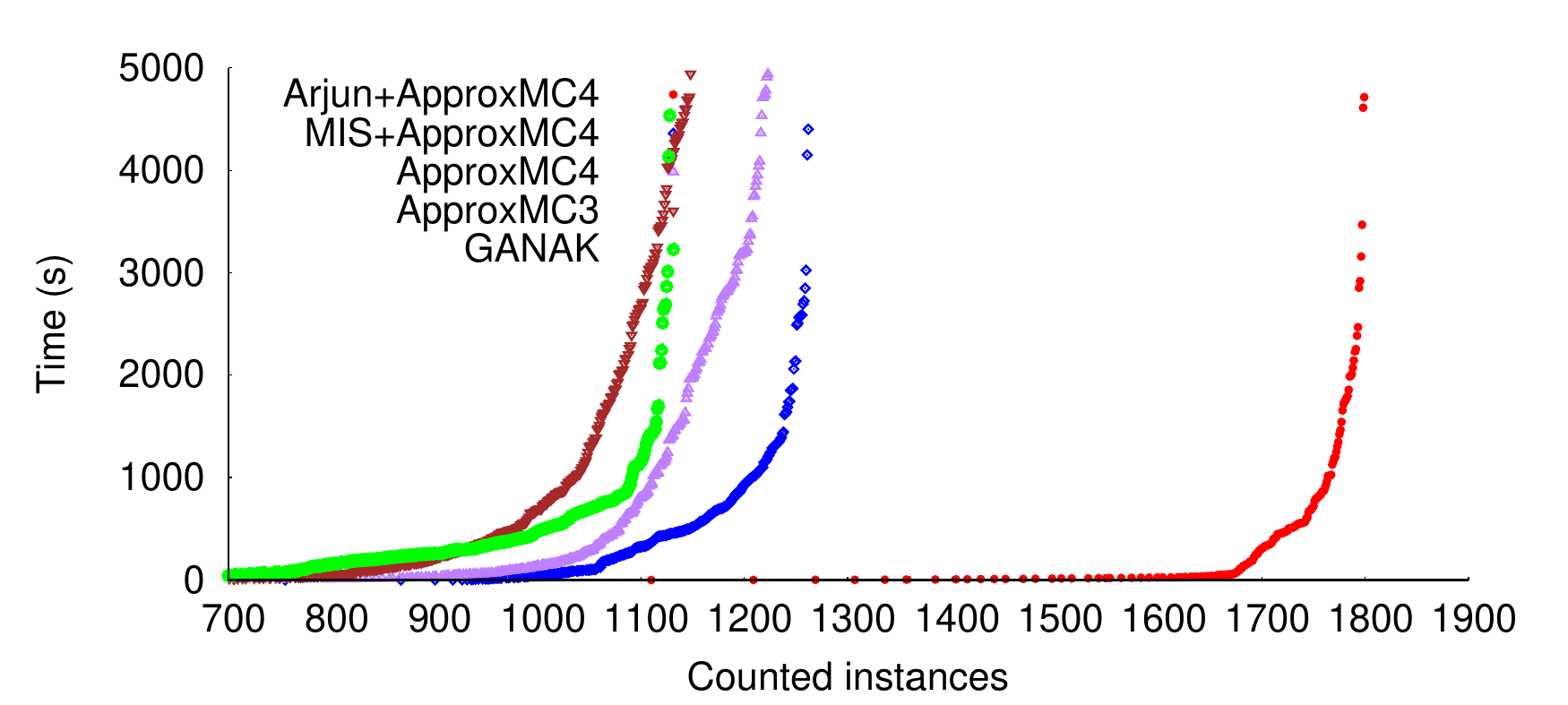
Basically, we can count in 2.24 seconds with Arjun+ApproxMC4 as many instances as we could count in 5000s with ApproxMC4 alone: more than 3 orders of magnitude improvement. In fact, it’s so fast we’ll need to switch away from our set of benchmark instances, because we are getting close to the limit of 1896, the number of instances in total. Notice that over the years, ApproxMC has improved dramatically in speed. In fact, the earliest ApproxMC could only count ~400 instances within 5000 seconds. We can now count 400 instances within a time limit of only 0.09 seconds.
Conclusions
As it may be evident from winning a number of tracks at the Model Counting Competition, Arjun is not only making ApproxMC faster — we also won the non-projected exact(!) model counting track with an entry called Arjun+SharpSAT-td, where SharpSAT-td [PDF] is an exact model counter by Tuukka Korhonen and Matti Jarvisalo. We hope to improve Arjun further in the future, and we hope Arjun will be become a standard preprocessor for model counters in the Model Counting Competition in the coming years, exploiting its CNF reduction capabilities that are currently available as: “./arjun input.cnf minimized.cnf”, using code and ideas from SharpSAT-td.