Probabilities of certain events are really hard to estimate sometimes. Often, it’s because we lack information of the underlying causal chains, but sometimes, it’s because the causes are so intertwined that even if we know the underlying probabilities of certain events happening along with the causal chains, it’s still impossible for us to untangle the web.
Let’s say there’s an event X has a probability of 0.4, Y has a probability of 0.6, and Z happens if either X or Y happens, but X and Y can’t happen at the same time, with a probability of 0.8. What’s the probability of Z happening?
The solution is easy to compute if you know how to use propositional model counters. They allow you to create a set of rules, such as:
X = 0.4
Y = 0.6
X or Y = True
0.8 -> NOT (X & Y)
The above perfectly describes the probability landscape, by using “->”, i.e. implication (if the left side is true, the right side must also be true), and using “&” (i.e. logical AND). Basically, for Z to happen, X or Y has to happen. And with probability 0.8, they must not happen at the same time. To solve the above, we add a helper variable H1, that will allow us to translate the last equation into an implication:
X = 0.4
Y = 0.6
X or Y = True
H1 = 0.8H1 -> NOT (X & Y)
To translate this to propositional model counting, we can do the following, where “-” is negation:
weight X = 0.4
weight Y = 0.6
weight H1 = 0.8
X or Y = True
-H1 or -X or -Y = True
The highlighted lines are what’s call the Tseitin transformation, which basically means that when H1 is TRUE, (NOT X or NOT y) must be TRUE, i.e. at least one of them has to be FALSE, i.e. they can’t happen at the same time (but it’s possible that neither of them happens). The above is what’s called a conjunctive normal form, or CNF for short.
The model counting DIMACS representation (formal description here) of the above is:
c t pwmc
p cnf 3 2
c comment X = 1, Y = 2, H1 = 3
c p weight 1 0.4 0
c p weight 2 0.6 0
c p weight 3 0.8 0
1 2 0
-3 -1 -2 0
c p show 1 2 3 0
Which is a straightforward 1-to-1 translation of the above, except we have to tell the counter that this is a projected weighted model counting problem (“pwmc”) and that it has 3 variables, and 2 constraints (“p cnf 3 2”).
Solving with a Model Counter
Once you have a CNF representation, you can run a modern propositional weighted model counter to count the number of weighted solutions, i.e. the probability of Z. I recommend the one I develop, ganak (linux binary here, open source code will be available soon, ask me if you need it):
./ganak problem.cnf
c s type pwmc
s SATISFIABLE
c s exact arb float 5.68E-01
So Z has a probability of 0.568. This can easily be verified to be correct:
Which adds up the probabilities that the left fires (but not the right), the right fires (but not the left), and that both fire, but the conflict does not happen (with 1-0.8 probability).
Of course, the above is a rather simple problem. However, with the above steps, one can create arbitrarily complicated causal chains, with complex constraints between partial, or intermediate elements of the chain, conditional probabilities, etc. Although there are limits to scalability, it’s many-many orders of magnitude faster than anything by hand, or by some form of brute-force checking/estimation.
Use-cases
In certain scenarios, it’s really important to know what the probability of some event is. For example, if you want to run a hazardous process such as a nuclear reactor or a chemical plant, or you want to provide insurance for some complicated (financial) product, accurately computing the probabilities of bad events happening is extremely important. I think it’s rather obvious that nuclear plants have very complicated causal chains for bad events happening — and they tend to be intertwined. If the external power lines are damaged, then likely it’s a major event (e.g. earthquake) and you likely also lost the majority of your transport capabilities, and along them, much of potential external help.
Similarly, if you want to bet for/against market moves, where you know or have a good idea of the underlying causal chains and associated probabilities, you can build quant trading, or expert advice systems based on the above. In other words, weighted model counting is not only useful for party tricks. Complex probability chains with thousands of interdependent random variables can easily be analyzed using the above system.
After many years of work, I am very happy to present our new CNF model counting preprocessor, Arjun [PDF][static binary]. It improves upon our approximate model counter ApproxMC [static binary], and can be used as a stand-alone binary to preprocess CNFs for (projected) model counting . Usage is simple:
./arjun blasted_case110.cnf
c Arjun Version: 43b17ef5899c461b8e947b0f3ca286efcf71464c
c CMS SHA revision 9bf1d82a7b9fa5492cf4f0437cf7110b77ad7230
[..]
c [arjun] original sampling set size: 284
c [arjun] final set size:   15 percent of original: 5.2817 %
Here, Arjun took a CNF that had a projection set of 284 variables, and reduced it to an independent support of only 15 variables. Arjun is now part of ApproxMC by default. Let’s solve a problem with ApproxMC without Arjun:
./approxmc --arjun 0 blasted_squaring42.cnf.gz.no_w.cnf.gz
c ApproxMC SHA revision 9fb4fdd01b40cc0526c4933e2f2dca402f0ab91f
c CMS SHA revision 9bf1d82a7b9fa5492cf4f0437cf7110b77ad7230
c [appmc] Orig sampling vars size: 349
[after waiting 5000 seconds, it times out]
Now let’s do the same with Arjun (this does not use code from SharpSAT-td):
./approxmc blasted_squaring42.cnf.gz.no_w.cnf.gz
c ApproxMC SHA revision 9fb4fdd01b40cc0526c4933e2f2dca402f0ab91f
c CMS SHA revision 9bf1d82a7b9fa5492cf4f0437cf7110b77ad7230
c Arjun SHA revision 43b17ef5899c461b8e947b0f3ca286efcf71464c
c [appmc] Orig sampling vars size: 349
c [arjun] final set size:  155 percent of original: 44.4126 %
c [appmc+arjun] Total time: 12.80
c [appmc] Number of solutions is: 80*2**127
s SATISFIABLE
s mc 13611294676837538538534984297270728458240
Done in 12.8 seconds, NICE. Wanna try it out? Arjun+ApproxMC static Linux binary HERE, Arjun static Linux binary HERE. Research paper HERE. Arjun code HERE. Now that the demo is out of the way, let’s get into the nitty-gritty details!
Projected Model Counting
CNF model counting is the problem where you want to count the number of solutions to a set of equations written in the CNF form. This form is quite restrictive, but also very powerful, here is an example:
 x1 OR  x2 OR -x3 = True
 x1 OR -x2 = True
 x1 OR -x3 = True
 x1 OR -x4 = True
-x1 OR  x4 = True
The above set of constraints clearly have a solution, e.g. setting x1=True and x4=False will satisfy all constraints. The question in model counting is how many solutions a system has. The above problem has 5 solutions in total:
This was kinda easy. However, there are two complications. One complication tends to be is that there are a massive number of solutions. For example, there are 2^200 solutions. Enumerating them one-by-one is just not going to work. Hence, we need some smart systems to do the counting for us, that don’t count one-by-one. Secondly, often we are interested only in the distinct number of solutions over a certain set of variables. Let’s take the above example, and say we want the distinct number of solutions over variables x1, x2 and x4 only. So, let’s delete column for x3 from above table:
Notice there are only 3 distinct solutions: the rows marked with * are both the same, and the rows marked with + are also the same. This is called projected counting because we are projecting the solution space over a specific set of variables — in this case, x1, x2, and x4.
Computing the Independent set of a Projection Set
In the above example, our projection set was x1, x2, and x4. However, notice that x1=-x4, due to the constraints:
 x1 OR -x4 = True
-x1 OR  x4 = True
Hence, it is good enough to count over x1 and x2, since x4 is determined by x1 and so x4 cannot possibly make the distinct number of solutions smaller or larger. This realization is at the heart of calculating an independent support — we basically want to minimize the set of variables that we project over. The independent support is simply a subset of the projection set, that’s hopefully a lot smaller than the projection set.
An early work on independent support calculation is the B+E preprocessor [PDF], which aims to do two things: “B” which finds a small independent support, and “E”, which eliminates variables from the problem. Let’s concentrate on “B” here. In the B+E paper, the authors talk about independent support over all variables of the formula, not over a projection set. In other words, their code and paper originally was conceived to minimize a projection set that had all variables inside. In our case, their work would minimize x1..x4, finding that x1,x2,x3 is an independent support of x1..x4.
Implicit Definability
The trick of B+E is to use the idea of so-called implicit definability. Implicit deniability is really simple. If I take x1, x2 and x3, does that define the value of x4? Yep. In fact, x1 on its own would define the value of x4, because x1=-x4. However, sometimes you have equations that define a variable through a (large) number of other variables. For example:
 x30 OR -x10 OR -x20 = True
-x30 OR  x10 = True
-x30 OR  x20 = True
This set of constraints describe x10 AND x20=x30. In this case, x10 and x20 together define x30. So if you have the above set of constraints in a CNF, and you have x10, x20, and x30 all in your projection set, you can confidently take out x30 from the set — and the number of distinct solutions projected will not change.
Implicit definability states that we can find these definitions in an implicit way, using a relatively straightforward system. We make two copies of the CNF, let’s call these CNF1 and CNF2. Then, we have variables v1…vN in the first CNF and w1..wN in the second CNF. Now, we create new variables called indicator variables, i1…iN that indicate whether v1=w1, v2=w2… etc. After this setup, the query is simple. Given i1=TRUE (i.e. given v1=w2), is it possible that v2 is different from w2? If it is, then our new independent set must contain both i1 and i2 (If not, we can get rid of i2). Now we move to i3. Let’s set i1=TRUE and i2=TRUE, and ask if it is possible that v3 is different from w3? Otherwise, our independent set remains i1, and we ask, is it possible that i1=TRUE and i2=TRUE, but v3 is different from w3? etc. This way, we test all the variables from v/w1…v/wN, and eventually end up with a set of indicator variables that tell us a minimal independent support.
Explicit Definability
As an external observer, without knowing nothing about implicit definability, CNF copying and renumbering and the like, it is quite easy to figure out that x1=-x4 just by looking at the CNF, since it contains:
 x1 OR -x4 = True
-x1 OR  x4 = True
Such set of constraints can be trivially found using Tarjan’s algorithm. This is actually linear in the number of binary (i.e. 2-long) constraints, so this is super-quick to run. Similarly, we can very easily find the AND gate x10 AND x20=x30:
 x30 OR -x10 OR -x20 = True
-x30 OR x10 = True
-x30 OR x20 = True
It’s a quick check on all the constraints that are 3-long and have the corresponding 2-long constraints. Such syntactic checks are well-known parts of SAT solvers. For example, the extremely successful kissat solver has the following lines of code in gates.c:
if (kissat_find_equivalence_gate (solver, lit))
  res = true;
else if (kissat_find_and_gate (solver, lit, 0))
  res = true;
else if (kissat_find_and_gate (solver, not_lit, 1))
  res = true;
else if (kissat_find_if_then_else_gate (solver, lit, 0))
  res = true;
else if (kissat_find_if_then_else_gate (solver, not_lit, 1))
  res = true;
else if (kissat_find_definition (solver, lit))
  res = true;
So, kissat finds equivalence gates (i.e. x1=x2), AND gates (like x10 AND x20=x30), IF-THEN-ELSE gates, and curiously… “definition” gates. What could these be? Well, it turns out kissat uses a very cool trick to find definitions. It takes all constraints that contain a variable, say x30/-x30, and cuts off the x30/-x30:
-x10 OR -x20 = True  <-- we cut of "x30 OR"
x10 = True           <-- we cut of "-x30 OR"
x20 = True           <-- we cut of "-x30 OR"
Notice that this set of constraints is now unsatisfiable. In fact, for all gates that define a variable, if you take all the constraints that the variable is in, and you chop off the variable, the constraints will together be unsatisfiable. To find such gates, kissat uses a SAT solver called kitten. Kitten solves these problems really fast and allows for UNSAT core extraction (not present in kissat) to find the defining variables.
Arjun
So what did we do with Arjun? We basically do the following set of improvements over B+E — while not even once looking at B+E’s code, since it was close-sourced, and by the time the authors open-sourced it, we already had our paper in the review queue:
We allow taking in a projection set, rather than the full set of variables like B+E does. This allows us to compute and independent support of a projection set, which is extremely important for our model counter ApproxMC. With a small independent support, ApproxMC uses a smaller matrix, so Gauss-Jordan elimination, which is an O(n^3) algorithm in our implementation, is significantly faster.
We use CryptoMiniSat to our advantage to simplify the CNF formula before running explicit or implicit definability detection. CryptoMiniSat is a powerful system that allows fine-tuned set of heuristics to be run, completely controlled from the API, e.g. “auto str = string(“intree-probe, occ-backw-sub-str, distill-bins, “); solver.simplify(NULL, &str);”
We use all the different ways to syntactically recover gates: and/or gates, if-then-else gates, and parity (XOR) constraints. We also recover gates semi-syntactically using picosat (instead of kitten) — this is semi-syntactic, because we use syntactic methods to get the occurrence list of a variable and to construct the SAT query, but then use a SAT solver (i.e. a semantic method) to recover the definition, if any. We then construct a directed graph from the gates and greedily find a minimum cover. This is needed because there could be loops, and we don’t want x1 to be defined by x2, and x2 being defined by x1, and accidentally remove both, which would be silly.
We repeat steps 2 & 3 at least 2x to make sure it’s done to a good enough level. This allows us to save time on the expensive next step, implicit definability detection. At this stage, we also do empty occurrence detection — if a variable is in the projection set, but doesn’t even occur in the formula, then obviously the variable can be removed and the count increased by a factor of 2.
We change the SAT solver’s assumptions method to improve implicit definability detection. From the standpoint of a SAT solver, the queries mentioned in the implicit definability section are so-called assumption queries: assuming i1=TRUE, v2=TRUE, v3=FALSE, is there a solution? The list of assumptions tends to be very long here, so SAT solvers can struggle. Our insight here is to change the traditional way of how assumptions are handled in the SAT solver, and effectively make the SAT solver not backtrack to the beginning every time a query is made. This makes quite a bit of difference in performance.(Note: it turns out this improvement idea has been invented, and re-invented, a few times already, e.g. by SharpSAT-td, and by IntelSAT — see Alexander Nadel’s presentation at SAT 2022).
That’s all folks! These improvements add up to about 5k LoC of code. All in all, they make Arjun more than an order of magnitude faster than B+E, and it can compute an independent support over a projection set, rather than all variables in the formula.
Performance of Arjun
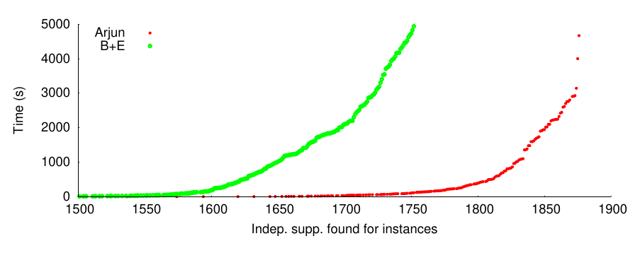
Here’s an example performance graph for B+E vs Arjun, using the set of benchmark instances we have been measuring the performance of ApproxMC on for ~5 years now — perhaps outdated, but at least it’s easy to compare all the values in all of our papers. The performance difference is quite big:
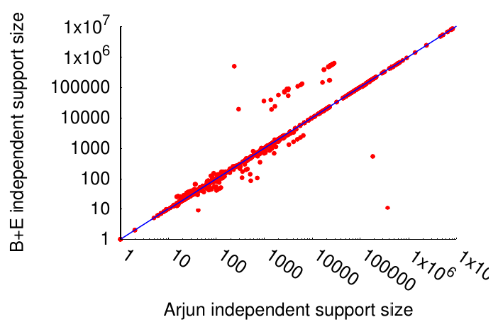
Basically, in B+E took 4932 seconds to compute the independent set of 1752 instances, while Arjun did the same in 117 seconds. Quite nice, about 40x improvement. Notice that due to the way our implicit definability works, it’s possible to e.g. order the variables in such a way as to make querying faster, but end up with a larger independent set. So, here is the comparison of independent sets computed by the same system as per the graph above:
Essentially, the same, modulo some noise. There is some advantage to using B+E in a few cases, and there is some advantage using Arjun in other cases, from the perspective of the calculated independent set. However, notice that Arjun is so much faster, that we could actually run it 2x with different variable ordering, thereby getting a (much) smaller independent set, and often still be a lot faster than B+E. However, there is always a trade-off, so we decided to be approximately as good in the minimization as B+E, while being significantly faster.
Performance Impact on ApproxMC
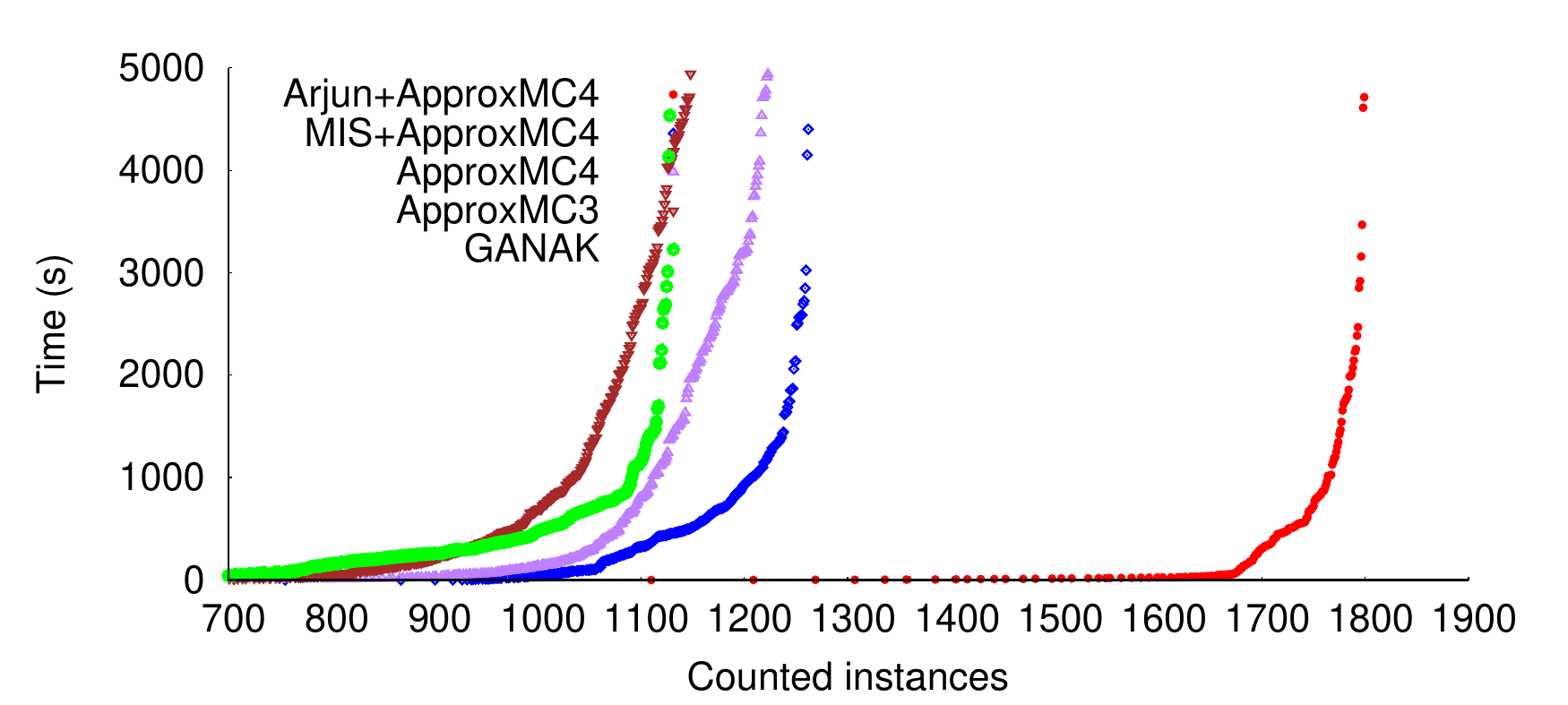
So, Arjun is fast but what does that mean for ApproxMC? It turns out, it means a lot. ApproxMC adds XOR constraints over the projection set, and the smaller the projection set, the smaller the XORs . Hence, the matrix that the Gauss-Jordan elimination algorithm has to run on inside ApproxMC is much smaller — which is an O(n^3) algorithm in our implementation. Hence, the performance of ApproxMC4 vs Arjun+ApproxMC4 is remarkable:
Basically, we can count in 2.24 seconds with Arjun+ApproxMC4 as many instances as we could count in 5000s with ApproxMC4 alone: more than 3 orders of magnitude improvement. In fact, it’s so fast we’ll need to switch away from our set of benchmark instances, because we are getting close to the limit of 1896, the number of instances in total. Notice that over the years, ApproxMC has improved dramatically in speed. In fact, the earliest ApproxMC could only count ~400 instances within 5000 seconds. We can now count 400 instances within a time limit of only 0.09 seconds.
Conclusions
As it may be evident from winning a number of tracks at the Model Counting Competition, Arjun is not only making ApproxMC faster — we also won the non-projected exact(!) model counting track with an entry called Arjun+SharpSAT-td, where SharpSAT-td [PDF] is an exact model counter by Tuukka Korhonen and Matti Jarvisalo. We hope to improve Arjun further in the future, and we hope Arjun will be become a standard preprocessor for model counters in the Model Counting Competition in the coming years, exploiting its CNF reduction capabilities that are currently available as: “./arjun input.cnf minimized.cnf”, using code and ideas from SharpSAT-td.
If you have a look at a modern SAT solver, say kissat or CryptoMiniSat, you’ll see that they have well over 20k lines of code. Reviewing that for bugs is basically impossible. So how can you trust that the solver is giving a correct result? Well, if the result is that the input formula is satisfiable, it’s quite easy — we can simply substitute the solution (all modern SAT solvers provide a satisfying assignment) to the formula, and it should satisfy each constraint. This is really fast to do, linear in the size of the formula.
However, if the solver gives a result that the formula is unsatisfiable (UNSAT), what do we do? Well, we need some form of assurance. One would be to check the code, but again, that’s just too much work. We could run it with another SAT solver, but there have been cases of the same bug being in more than one solver. Actually, this bug seems to have been a conceptual mistake copy-pasted, quite weird. In fact, there is a well-known GCC version that will miscompile most MiniSat-based SAT solvers such that they report wrong results(!). We could also do some fuzzing, but do you want to sit on an airplane knowing its flight control software was fuzz-tested for a full 10 minutes to “meet” compliance requirements? No. We need strong assurances. So, let’s ask the SAT solver to produce a proof for the UNSAT result! This is what proof traces are all about.
The Binary Resolution Operator
At its core, a proof trace essentially records the set of operations that must be performed by a system to arrive at the 0=1 equation (i.e. at obvious nonsense), starting with the input equations. Let’s see a simple example. Let’s have our input formula (so-called CNF) be:
 x1 V  x2 = TRUE
 x1 V -x2 = TRUE
-x1 V  x2 = TRUE
-x1 V -x2 = TRUE
Where x1 and x2 are boolean variables. Actually, let’s make this a bit easier to read by a computer:
 1  2 0
 1 -2 0
-1  2 0
-1 -2 0
This the same as the above, but closer to the standard DIMACS format. Each line is called a clause, each line is made up of literals like 1, -1, 2, and -2, and each clause is terminated by a “0”, marking the end of the clause.
The above CNF has no solution to its set of clauses: no matter what we set x1 and x2, at least one of the clauses is not satisfied. OK, so how do I prove that there is no solution? Well, the easiest way to do it is through the binary resolution operator. The binary resolution basically says that if two clauses have one literal that’s inverted, such as “x1” and “-x1”, then we can do this: (A OR x1) RESOLVE (B OR -x1) => A OR B, where “A” and “B” are any set of literals. So, e.g. “x1 V x2 V -x3” resolved with “x3 V x4” becomes “x1 V x2 V x4”. Nice, so let’s try to prove that the above problem is unsatisfiable:
In essence, we resolved 2 clauses to prove that x1 is TRUE, then resolved another two to prove that x1 is FALSE, and then we resolved “x1” with “-x1” to arrive at EMPTY=TRUE, i.e. 0=1, which is obviously nonsense.
The RUP notation
In the so-called RUP notation (“Reverse Unit Propagation”), the above is simply written as:
a  1 0
a -1 0
a 0
Basically, we simply write down each derived clause one after the other as “added” (=”a”). It’s called Reverse Unit Propagation, because it’s possible to prove each of these clauses to be correct, by starting from the top, and performing simple propagation [where propagation is substitution of the values into the equations, and checking if any variable is forced to a value] . Let me explain. Say we want to prove “1 0” is correct. Then, we set all the literals’ inverted values, here, “x1=FALSE”, and propagate on the original clauses plus any clause that’s above “1 0” (and hence has been proven to be correct). If we set x1=FALSE, then the original formula’s clause “1 2 0” will propagate x2=TRUE and then the original formula’s “1 -2 0” conflicts immediately (all its literals are now FALSE). Hence, propagation lead to a conflict! This means that indeed, “1 0” must hold.
What’s important to realize here is that each of the lines of the proof must be checkable by simple propagation. Let’s say we have this set of constraints:
8 9  2  3 0
8 9 -2  3 0
8 9  4 -3 0
8 9 -4 -3 0
Given these constraints, it is fairly easy to check that “8 9 0” holds. However, we can’t just write into the proof that “a 8 9 0”. Because for that, the propagation check as explained above should succeed: when I set both x8=FALSE and x9=FALSE, I should get the a conflict. But I don’t! Instead when I substitute x8=FALSE and x9=FALSE in to the equations, I get this reduced formula:
 2  3 0
-2  3 0
 4 -3 0
-4 -3 0
Which does not force any variable to any value (i.e. they don’t propagate anything) and none of them are the empty clause, so I’m stuck. The proof verifiers literally will say they are “stuck”. So, how I can prove “x8 OR x9”? Let’s do it like this:
a 8 9 -3 0
a 8 9  3 0
a 8 9 0
Let’s see how this works. First, let’s try to validate “8 9 -3” by setting v8=FALSE, v9=FALSE, v3=TRUE. Then the original constraint “8 9 4 -3 0” will propagate v4=TRUE, and the original constraint “8 9 -4 -3 0” will be immediately conflicting (all its literals are now FALSE). So simple propagation fails, hence the clause “8 9 -3” must be correct. While this is not the goal (that’s “8 9 0”), we are getting there. We now prove “8 9 3” in a similar fashion, and then we prove “8 9 0” in the same fashion. Easy!
Faster Proof Verification: DRUP
While RUP is indeed a good format, we don’t always need all the constraints to be in the active set in order to prove UNSAT. Let’s quickly re-visit this CNF, and try to prove “8 9 0”:
8 9  2  3 0
8 9 -2  3 0
8 9  4 -3 0
8 9 -4 -3 0
In order to reduce memory load, let’s delete all the clauses we don’t need after we used them! These steps are going to be noted with “d” (=”delete”) instead of “a” (“add”):
a 8 9 -3 0
d 8 9  4 -3 0
d 8 9 -4 -3 0
a 8 9  3 0
d 8 9 -2 3 0
d 8 9  2 3 0
a 8 9  0
d 8 9 -3 0
d 8 9  3 0
NICE! So we first derived “8 9 -3 0” and then removed both of the clauses we used to create it, they are not needed anymore! Begone “8 9 4 -3 0” and “8 9 -4 -3 0” ! Same thing with “8 9 3 0”. Then, once we derived “8 9 0”, we even deleted the intermediary constraints “8 9 -3 0” and “8 9 3 0” we previously derived. Begone! Not needed anymore, all we need is “8 9 0 “.
Extended resolution for proofs
Okay, I’m gonna cut this part short, mostly because I am terrible at this, but we have talk about the elephant in the room: RAT, or, more beautifully, Resolution Asymmetric Tautologies. So, what is it? Essentially, it allows you to declare new variables in your proof and use them later. This is absolutely amazing, because with this, you can provide so-called extended resolution proofs (warning: 1968 research paper), which allows us to express certain proofs more compactly, in fact, exponentially more compactly!
Here’s how to do it. Let’s say you want to use the definition “x1 OR v2 = x99” in your proof, because it would make your proof smaller. This can happen, for example, because your constraints often have “x1 OR x2” in them, and now you can replace all of those parts with simply “x99”. Well then, you write this into your proof file:
a -99 2 1 0
a  99 -1 0
a  99 -2 0
Notice that this is just a simple OR gate definition. The only thing RAT requires is that (1) the first variable is the one that’s being defined and (2) the introduced variable must not be part of our input formula — so our input formula here should have at most 98 variables. That’s it. Now you can use x99 anywhere you like, as long as it makes sense. For example, you could take a clause “1 2 3 4 0” and convert it to “99 3 4 0”:
a  99 3 4 0
d  1 2 3 4 0
Notice that “99 3 4 0” is simply a RUP proof at this point: setting 99=FALSE, 3=FALSE, 4=FALSE will immediately propagate x1=FALSE, x2=FALSE (due to the clauses “99 -1 0” and “99 -2 0”), and x1,x2,x3, and x4 all being FALSE will immediately trigger a conflict for clause “1 2 3 4 0”, so we have the RUP property and we are fine. Then we can delete “1 2 3 4 0”, we don’t need it no more. Notice that I can’t write the reverse:
d  1 2 3 4 0
a  99 3 4 0
If I wrote that, “a 99 3 4 0” will not work, since it relies on “1 2 3 4 0” but we already deleted that, oops!
Besides the above trivial example with the OR gate, extended resolution can simulate, in polynomial time, some algorithms that are extremely hard (read: exponentially hard) for normal resolution to express. This means that using RAT, we can express even complicated mathematical concepts in this extremely simple system, for example in this case, pseudo-boolean reasoning.
What the solver does vs. what the proof checker does
So let’s say you implement DRAT proof trace into your SAT solver and your proofs are always verified. All good! Not so fast. One day you decide to check the proof that DRAT recovered, and to your absolute horror, you realize that DRAT thinks your proof to be substantially different than what the SAT solver thought it was! How can that be?
Well, the DRAT checker recovered a proof. It’s a valid proof, and it can be recovered given the set of clauses that haven’t been deleted using the “d” operator, as above. But notice that we never told the proof checker which set of clauses we resolved on to get to a clause! It just kind of figured it out by itself. Now, we can look at this and say, this is great because (1) I don’t have to do hand-holding of the proof checker, and really interestingly, (2) the proof checker could actually recover different proofs from the same proof trace(!). Ambiguity can be useful. Well, that’s great, but what if I really-really want to know what the SAT solver actually did?
Enter FRAT. This proof format is super-close to DRAT, with the following changes. Firstly, FRAT numbers each clause with a unique clause ID. This is needed because the same clause can be in the solver’s memory more than once, and we need to be able to distinguish them from each other — they may have been derived in completely different ways! Secondly, FRAT allows an optional hint at how the clause was derived. Let me give a hands-on example, it should be quite clear. As a reminder, here is the input formula we had before:
 1  2 0
 1 -2 0
-1 -2 0
-1  2 0
And here is the DRAT proof:
a  1 0
a -1 0
a 0
Now, for the FRAT proof:
o 10  1  2 0         -- input clause, let's set its ID to 10
o 11  1 -2 0         -- input clause, let's set its ID to 11
o 12 -1  2 0
o 13 -1 -2 0         -- last input clause
a 14  1  0 l 10 11 0 -- first resolvent
d 10  1  2 0
d 11  1 -2 0
a 15 -1  0 l 12 13 0 -- second resolvent
d 12 -1  2 0
d 13 -1 -2 0
a 16 0 l 14 15 0     -- empty clause! It's UNSAT!
f 14  1  0           -- finishup from down here
f 15 -1  0
f 16 0
Okkkay. So… the original clauses are part of the proof trace now, they start with “o”. And each clause has an ID, after o/a/d/f. This can be any number, but they must be non-clashing (obviously). Furthermore, we are allowed to have an “l” after the closing “0” when adding a clause — these are the clause IDs we had to resolve to arrive at the new clause. So, e.g. IDs 10 and 11, i.e. “1 2 0” and “1 -2 0” must resolve to “1 0” (clause ID 14). And finally, we must “finalize” all our clauses, i.e. we must account for all clauses remaining in memory, with the “f” command.
Firstly, finalization means that in case your SAT solver forgot to delete a clause in the proof trace, but deleted it from memory, finalization will fail, because the solver will not finalize that clause, and so the checker will complain. In essence, finalization forces the hand of the SAT solver writer to make sure that the “view of the world” from the perspective of the SAT solver and that of the proof verifier match when it comes to clauses in memory. This is not the case for DRAT — the proof verifier there could have millions of clauses more in memory than the SAT solver :S
Secondly, the “l” notation means that we can now be precise about what clauses were actually resolved by the SAT solver to arrive at a new clause. However, this is only a “can” — adding the “l” is not necessary, and of course can be stripped. This means that if we want to, we can have ambiguity, or if we want to, we can have precision. The best of both worlds!
Trusting trust
Proofs are cool, and are very important so we can be sure our results are correct. But… are we sure they are correct? Well, not so much. You see, the proof verifiers themselves are not verified. Say, frat-rs will say “VERIFIED” on a FRAT proof, but… frat-rs itself is over 5000 lines of Rust. And before you think I’m really stretching things here, let me just remind you that I personally found a segmentation fault in drat-trim, the official DRAT proof verifier, used at the SAT competition. (I actually found the bug accidentally while fuzzing my own SAT solver.)
So, what can we do? Well, we need another verifier. I’m not kidding. Basically, frat-rs can take a proof that the SAT solver provides, and translate it to a fully annotated, clean proof with all the deletions at their earliest possible points (see this hack). We can then write a slow, but verified proof checker, that can do the trivial checking that the resolutions are indeed correct, reaching the empty clause (i.e. 0=1). The pipeline would then be:
What this allows us to do is that we don’t need to trust the SAT_solver or frat-rs. We can treat them as black boxes. All we need to trust is that the verified_proof_checker is correct: given the SAT_query, the solution can be trusted. In this sense, clean_proof is simply a hint for the verified_proof_checker to do its job. Notice that I completely skipped how SAT_query can be trusted — that’s an entirely different can of worms :D
In case you want to use such a verified proof checker, there is one in lean4, available here, and one for acl2, available here. The non-verified tool to “elaborate” simpler (e.g. DRAT) proofs into annotated (LRAT) proofs, you can use frat-rs.
Conclusions
So, we talked a lot about proof traces, proof formats, and how to trust the solution. In some cases, this is extremely important — some software and hardware is verified in this way that controls trains and airplanes, and industrial systems (think: nuclear reactors, rockets… Ariane 5 crash anyone?). We certainly don’t want any bugs in there.
What I didn’t talk about, is that proof traces do something else, as well: they allow us to understand how SAT solvers work. You see, while the proof is written in the forward fashion — the same direction that SAT solvers work, — the proof actually only makes sense in the reverse direction. We always start at the empty clause, at the end of the proof, and walk backwards to see how the empty clause got proven! So, if you think about it, proofs can be used to look at SAT solvers in the reverse direction. And that’s super-exciting. For example, how much work did the SAT solver really have to do to reach the empty clause? How much complete nonsense did it do that was utterly useless to prove unsatsifiability? How many times did it forget proof fragmets that it later had to re-learn? Or, what is the minimum memory footprint that its produced proof could fit in? And if we take advantage of DRAT’s and FRAT’s ambiguity: is there a proof with fewer steps it could have produced given the total same set of resolvents? In my opinion, there is a whole wealth of data in proof traces that we should do research on to learn more about SAT solvers.
(PS: Tracecheck is one of the earliest proof trace systems. I didn’t want to mention it because it’s not as relevant anymore as the above, and it would have made the story a tad more confusing)
This blog post is to promote the tool here (paper here) that converts weighted counting and sampling to their unweighted counterparts. It turns out that weighted counting and sampling is a thing. It’s basically a conjunctive normal form formula, a CNF, with weights attached to each variable. One must count the number of solutions to the CNF, where the weight of each solution is not necessarily 1, but weighted according to the polarity of each variable in the solution. One such formula could look like:
p cnf 2 1
c ind 1 2 0
1 2 0
w 1 0.9
This basically says that we have 2 variables, a single constraint (“v1 or v2”) where a solution with v1=True is worth 0.9 points, but a solution with v1=False is only worth 0.1 points. Or, if we are sampling, we want to bias our samples 9-to-1 for solutions that have v1=True.
Let’s go through this CNF. It has has 3 solutions, with its associated points:
The issue is that we have great tools for doing unweighted counting and sampling but few tools for doing weighted counting and sampling.
Converting Weighted CNFs to Unweighted CNFs
The solution is to use a converter to make an unweighted formula from a weighted formula, and then either divide the number of solutions of the unweighted formula (for counting) or simply cut off variables from the samples (for sampling). This work was done by Chakraborty et al. and presented at IJCAI’15. The basic idea is that we can approximate the weight with a binary representation and encode that in CNF. For example, 0.26 can be approximated with 1/4. If this weight is attached to v1, and there are 10 variables in the original CNF, we generate the extra set of clauses:
12 -1 0
11 -1 0
12 -11 1 0
This CNF has exactly 1 solution when v1=True and 3 solutions when v1=False. So the number of positive solutions is 1/4 of all solutions, i.e. 0.25, close to the requested 0.26.
The above set of clauses is generated from chain formulas that can be easily generated, and are only polynomal in size of the binary precision required. For k-bit precision (above: 2 bit precision), we need only k extra variables and k+1 clauses. See the paper for details, but it’s sufficient to say that it’s easy to generate and, looking through a few examples, quite easy to understand.
Example: Weighted Counting
Let’s do the full run, using our favorite counter, approxmc:
$ cat my.cnf
p cnf 2 1
c ind 1 2 0
1 2 0
w 1 0.9

$ ./weighted_to_unweighted.py my.cnf my-unweighted.cnf
Orig vars: 2       Added vars: 7
The resulting count you have to divide by: 2**7

$ ./approxmc my-unweighted.cnf
[…]
[appmc] FINISHED AppMC T: 0.01 s
[appmc] Number of solutions is: 62*2**2

$ python
>>> 62*2**2/2**7
1.9375
So, we got pretty close to the correct weighted count of 1.9. The reason for the discrepancy is because we approximated 0.9 with a 7-bit value, namely 115/2**7, i.e. 0.8984375, and we used an approximate counter. With an exact counter such as sharpSAT, we would have got:
And we are done! The sampling worked as expected: we get proportionally more samples where v1 is True than when it’s False.
Conclusions
Weighted counting is non-trivial but can be approximated using chain formulas, blowing up the original equation in only a minor way. This allows us to use well-optimized unweighted systems to perform the counting and sampling, and then trivially transform the output of these tools to match our original weighted problem.
This is going to be a long post, collecting many years of work, some of which was done by my colleagues Kuldeep Meel and Raghav Kulkarni. They have both significantly contributed to this work and I owe a lot to both. The research paper is available here (accepted to SAT’2019) and the code is available here. Build instructions are at the bottom of the post. Part 2 will deal with exploring the data in more detail.
I always had a fascination with data when it comes to SAT solving. My SAT solver, CryptoMiniSat always had very detailed stats printed to the console. At one point, this fascination with data got to the point where tallying up data from the console (with AWK, like a true hacker) didn’t cut it, and I started dumping data to SQL.
An Early Attempt: Visualization
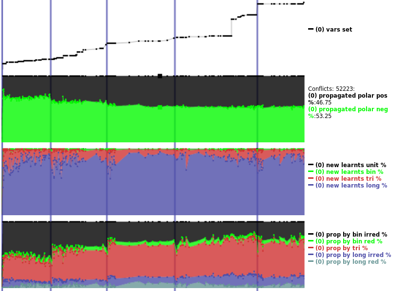
Out of the SQL data dumped, this website was born, back in 2012. This site displays pretty graphs like:
These graphs can show quite a bit of data, the above must be a few hundred data points. The data gathered is pumped to an SQL database, and then visualized. I felt like I am on to something. Finally, I was going to be able to explain things.
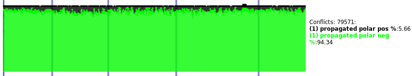
But I was able to explain very little. Some things were quite obvious, like how industrial and cryptographic instances’ variable polarity distributions were so different. Above, the black/green graph shows a cryptographic instance, and the distribution is 47% vs. 53%. On a typical industrial instance, the same graph looks like:
Here, the polarity distribution is 6% vs 94%. This is easy to see with the human eye. But I was gathering tons more data, many megabytes per instance. What was I going to do with all this data? How was I going to know what is good and bad behavior? And how would I make the solver work towards good?
SATZilla: Solver Selection Using Machine Learning
I wasn’t the only one trying to make sense of SAT-related data and improve solving based on it. SATZilla has done this before. There, the idea was to gather information — called features — about the input CNF problem, run multiple SAT solvers, save how much time it took for the solver to run, then create code that matches the CNF features to the preferred SAT solver. This creates a lines like:
Where the first N columns are the features and the last column is the label that we calculated to be correct. SATZilla uses many features, such as the number of horn clauses, the ratio of variables and clauses, etc. Once such a table has been built, with lines called labeled training examples, it uses a machine learning system, for example Decision Trees, to classify (i.e. guess) which SAT solver would be best for any CNF instance. So it generalizes, and can guess which SAT solver is best for a CNF it has never seen.
This system is interesting but has some drawbacks. First, for each data line one must run 5-10 SAT solvers on a CNF, potentially using up to 20-30’000 CPU seconds. Hence, each labeled training example is extremely expensive. If you know about the Big Data hype, you know that spending $2 on a single data point is not viable. Modern systems use millions of labeled training examples to learn a classifier. Secondly, this system was not designed to work in an industrial setting, where the CNF is not presented in a single file but piece-by-piece through a library interface.
Enter DRAT
DRAT is a system used to verify the resolution proof that modern SAT solvers generate. Basically, every unsatifiable problem that SAT solvers solve can be shown to be unsatisfiable through a set of operations called resolutions, that eventually lead to the equation 0=1, which is trivially false. A DRAT verifier can know exactly which clause was used by the SAT solver at exactly which time during the creation of the proof. Hence, DRAT knows a lot. It can actually tell, after the solving has finished, which parts of the SAT solving were absolutely useless, and which ones useful. A resolution proof with thousands of resolutions can be computed in seconds, which means cheap data.
When I first really understood DRAT, I realized, what if I could get all this data out of DRAT, and use it as a label for the millions of data points I already have? I have finally found a label, available at a huge scale, to train on.
The Beginnings of CrystalBall
What to train for was still a question that needed answering. Since DRAT is so intimately connected with learnt clauses, I decided to train for throwing away as many unneeded learnt clauses as possible. This would definitely make solving faster, by throwing away everything that is useless weight and making sure everything that is useful stays.
I must thank Marijn Heule who helped me with the first hack of DRAT-trim in early 2016 to get data out from from it. I hacked CryptoMiniSat to add Clause IDs to DRAT, so the verifier, DRAT-trim, could read and track these IDs. I now knew which clause was used in the proof and which wasn’t. This sounds really useful — you could now know which learnt clauses should have been thrown away the moment they were generated, since they were useless. Let’s see some data from modern CrystalBall (see at the bottom of the post how to download, compile and run):
sqlite> select count() from sum_cl_use where num_used>0;
51675

sqlite> select count() from sum_cl_use where num_used=0;
42832
The data says that about 50% of clauses were useful. Let’s see what is the average LBD value of the useful and useless clauses:
sqlite> select avg(glue) from sum_cl_use, clauseStats where sum_cl_use.clauseID = clauseStats.clauseID and num_used > 0;
6.71436865021771

sqlite> select avg(glue) from sum_cl_use, clauseStats where sum_cl_use.clauseID = clauseStats.clauseID and num_used = 0;
9.80162028389989
Nice. Let’s get the sizes, too, by replacing “glue” with “size”:
There are plenty more, well over a hundred, that is being measured, so I won’t bore you. I have a feeling you could write a few research papers just by running queries on this data.
I don’t know if you noticed, but something is odd here. SAT solvers only keep about 5-10% of all clauses. Just run a modern SAT solvers to completion and check how many clauses remain in the clause database. How is this compatible with 50% of clauses being useful? Well, we can use clauses for a while, then throw them away. But for that, we need much more than just whether a clause is useful or not. We need to know exactly when it was useful. Clauses can be used many-many times in a single proof.
We Need More Refined Labels
It turns out that having only whether a clause is being used is not good enough to compute useful labels. We need to know when, exactly, was the clause useful. So CryptoMiniSat and DRAT-trim was hacked to output into the DRAT proof exact conflict numbers when a clause was created. This, with some minor magic, would tell us exactly when each learnt clauses was used:
sqlite> select sum(num_used) from sum_cl_use, clauseStats where sum_cl_use.clauseID = clauseStats.clauseID and glue<=3;
332689

sqlite> select count() from clauseStats where glue<=3;
11221
For this problem, a clause that had LBD 3 or lower was used on average 332689/11221.0=29.65 times in the proof. Okay, how about clauses with LBD 4 or larger? It’s a trivial change in the above code, and gives us 5.95. Cool, the lower glue, the more it’s used in the proof.
Now that we know how to walk, let’s run. When was clauseID 59465 created and at what conflict points was it used in the proof?
sqlite> select conflicts from clauseStats where clauseID=59465;
101869

sqlite> select used_at from usedClauses where clauseID = 59465 order by used_at asc;
101870
123974
152375
This is an interesting clause. It was generated at conflict no. 101869, was used in the proof right after it was generated, at conflict no. 101870, and then it was used in the proof more than 20’000 conflicts later, twice.
The Data Pipeline
The idea is this: we are going examine every learnt clause at every 10’000 conflicts, and guess whether it’s going to be used in the future enough for it to be kept. If it’s going to be used enough in the future, we keep it. If not, we’ll throw it away. What do we need for this?
Well, we need a ton of labeled training examples. And for that, we need a truckload of data, one that generates so much that we have to throw away 96% and still end up with hundreds of MBs in under an hour. Also, we need this from a wide variety of problems, and we need to be able to debug the hell out of this data, because where there is tons of data, there are tons of NaNs, and negative clause sizes and the whatnot. So we need a data pipeline.
The first part of the pipeline we only run once, because it’s a bit expensive, about 3-10x slower than a normal CNF run, and looks like this:
Run CryptoMiniSat without any clause cleaning, and write an SQLite database with all dynamic data gathered. The data written is about: the CNF (such as number of claues, etc.), the restarts (e.g. avg. LBD, restart length), the learnt clauses (e.g. LBD, size), and at every 10’000 conflicts the dynamic characteristics of the learnt clauses (e.g. activity, number of times used in a conflict the past 10’000 conflicts)
Run DRAT, and dump all usage data to a file. Augment the SQLite data with the DRAT data
Sample the data because otherwise it’s going to be too much. We need to sample smartly, though, because without biased sampling, the really weird cases will not be represented in the final data at all, and our machine learning system will not see some really interesting data. If we could store and process 1TB of data (you can generate that rather easily), we wouldn’t have this issue. But we can’t.
So now we have a ton of cool data that is very raw. This is going to be our baseline. We’ll keep this data in our stash and never modify it.
The second part of our data pipeline will use this stash of data to do all the cool things we want. This 2nd part is much-much cheaper to run (few seconds to a few minutes per CNF), so we will be able to run it as many times as we like, playing with all the cool parameters. This second part of the pipeline will:
The data is stored normalized in SQLite for speed and space. For machine learning, we must denormalize it, to have everything related to decision on a single line.
Create the labeled training data using Python Pandas for easy data manipulation and visualization
Notice that this table has essentially two parts. The left part, i.e. everything apart from “keep”, called features, must be available to the solver during running. And the right part, “keep”, the label, which is computed using data from DRAT-trim. This latter the solver has no access to during running, this is our crystal ball, looking into the future. What we want is to predict the label given the features.
The left hand side, i.e. the features are not so difficult to do. Adding a new feature is now about 3-4 lines change in CryptoMiniSat and it’s essentially free in terms of speed. The data gathering only needs to run once (the 1st part of our data pipeline) and it is not running during solving. So, you can add as many features as you like. If they are useful, then you also need to add some lines to the solver so they will be available during running — of the 200+ only a few are really useful.
The right hand side, i.e. the labels are a completely different story, though. We know what is the future, kinda (yes, the future is a function of the past&present, but let’s not go there for the moment). So given the future, how do I label things? We need to use a heuristic. The good part is that we have a ton of information about the future, such as the distribution of all clause’s usage in the proof, and the number of times a particular clause is used in the future. But we still need to come up with something to decide KEEP/THROW_AWAY. A simple such heuristic is: if in the next 10’000 conflicts this clause will be used at least 6 times, keep it. Otherwise, into the bin it goes:
CASE WHEN
-- useful in the next round
   used_later10k.used_later10k > 5

THEN "keep" ELSE "throw_away"
END AS `x.class`
Nice! Remember that clauseID 59465 that I talked about above? Yeah, that would be labeled THROW_AWAY — it was only used 20’000 conflicts later. We have labeled our data, now we need to train a classifier, make it output C++ code and we are good to go. But before that, let’s play with Weka.
Data Analysis And Machine Learning with Weka
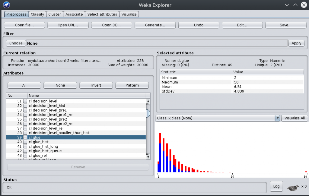
Weka is a cool tool for exploring data and building simple classifiers. You can get a free Weka course on Futurelearn, and I highly recommend it. The person who wrote it is the one who is giving the course and he is really cool. The denormalized, labeled data can be output to CSV (see at the bottom), which Weka can read:
Here, you have Weka showing the denormalized set of features on the left, and showing the LBD distribution on the right. Blue color is for for lines labeled KEEP and red color is for lines labeled THROW_AWAY. As you can see, the distribution of blue vs red is not the same at all as the LBD value increases (hence LBD being a good discriminator, see glucose).
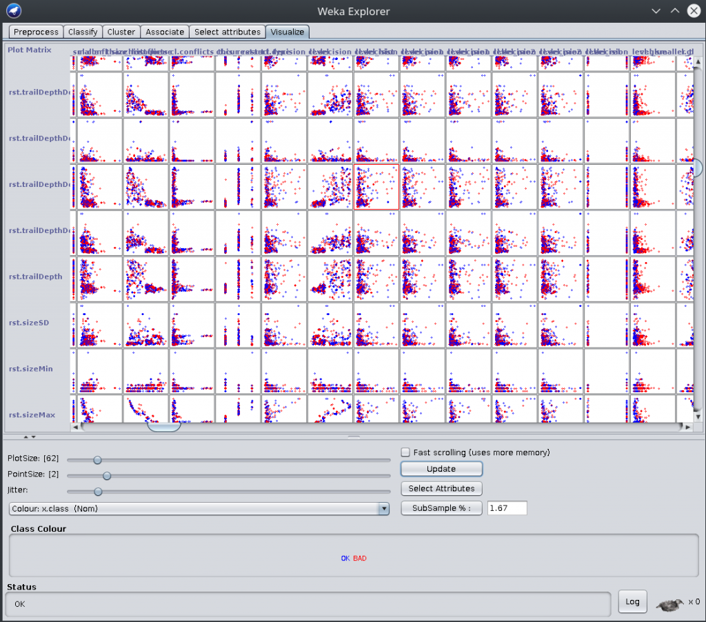
You can also visualize correlations:
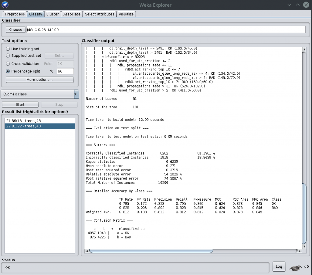
You can also build classifiers based on this labeled data. Just don’t forget to delete the “sum_cl_use.*” features, as they are not really features, they are data from the proof verification. If you don’t delete them, Weka will cheat and use them in the classifier, which is like using the solution key during the exam :) Let’s create a classifier using Weka:
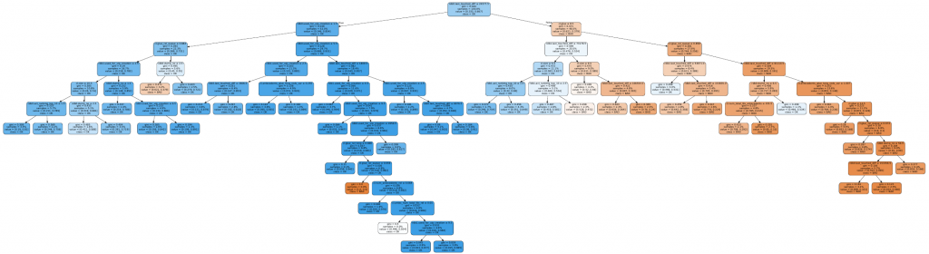
This shows a confusion matrix at the bottom. Nice. Total misclassification was 18% using the J48 decision tree algorithm with some minor tuning. Here is such an example decision tree (PDF here):
Weka is great in many ways, and I will forever be indebted to it. However, it’s just not gonna cut it for us. We need something a lot faster, and we need to be able to automate it and we need to be able to get C++ code out. Weka could do some of these, but I’m not a Java programmer, and Weka’s speed is nowhere near that of scikit-learn. However, if it’s your first time doing machine learning, Weka is an amazing tool.
Training a Classifier Using scikit-learn
Now that we have labeled training data, we need to create a classifier so that the solver, during running, can take the features it knows and guess the label KEEP or THROW_AWAY. There are many-many different classifiers that can be trained, and I have tried the most important ones, such as logistic regression,SVM, decision trees and random forests.
Let me pause here for a moment. If you haven’t done machine learning before, you might think — this is where the magic is. The classifier is where it’s at! And if you have done machine learning before, you know full well, it’s not here at all. It turns out that the quality and quantity of your data is way more important than the classifier you choose. It’s relatively easy to see why. If your data is messy, incorrect, or missing elements, no matter what classifier you use, no matter how amazing it is, it will give you bad results. Bad data, bad results. Every. Single. Time. Keep this in mind.
So, we have chosen our classifier, say, decision trees. Decision trees are easy to visualize, and you will need to debug the hell out of this, so it comes handy. After all, nobody wrote 1000 lines of python and it came out perfect the first time.
Now, there are still some things to deal with. First, we cannot possibly use all 200+ features in our prediction. We can generate the tables, but we need to be reasonable, and cut down the features to something much smaller, say, 20, during the running of the solver. To do that, we create a large random forest and then check which features were picked by the most trees. That gives us feature ranking (thanks to Raghav Kulkarni for this trick):
So the top 5 features for this particular run are these. For different instances or different configurations, the top features may differ, and you probably want to sample X number of labeled training example from each problem, put it in a large data file and then run the feature ranking.
There are still some minor obstacles to overcome. Since about 95% of the clauses need to be thrown away, our labels will be very unbalanced. So we need to balance that. Also, how aggressive do we want to be with throwing clauses away? Should we err on the side of caution? Note that this is not about labeling anymore. The label has already been chosen. It’s about guessing the label. We are now tuning what’s called the confusion matrix:
Here, we have 80% of things that we labeled as KEEP actually being guessed to be kept, while 20% of them are wrongly guessed as THROW_AWAY. So it’s kinda okay. We are better at guessing if something needs to be thrown away, though, there we only guess 5% of them wrongly. Maybe this a good balance, but if not, it can be changed as a weight parameter.
The system can also classify clauses into different types, using K-means clustering. Then it can train a different classifier for each clause type. The K-means clustering uses the already denormalized features, so it’s really trivial to do, though which features should be used for the clustering is a good question. I currently use the CNF features only (e.g. number of clauses, variables, ratio of vars/clauses, etc.), thereby clustering problems rather than clauses. One could could use any set of features though, it’s all automatic, including C++ code generation.
Actually, the C++ code generation. The system produces C++ code for decision trees, random forests and K-means clustering, ready for it to be compiled into the final executable. We have now created our clustering and classifier, and it’s all in C++ code. Let’s run it!
The Final Solver
This is the most fun part. And the cumulative effort of a lot of work. It’s really interesting to see all those thousands of lines of C++ and python churning out gigabytes of data, being boiled down to juts a few hundred lines of automatically generated if-then-else statements, running during solving. But there it is.
Let me talk about the good parts first. It’s very fast at evaluating whether to keep or throw away a clause. You don’t even notice it running. It doesn’t use much more memory than normal CryptoMiniSat (i.e. a few features were enough), and it correctly guesses the cluster where a clause belongs. It also guesses the labels correctly with very high probability. The final solver beats every solver from 2018 on the SAT competition 2014-17 instances.
Another great thing is that this system can be used to automatically train forspecific problem types. This can be very significant in industry, where the instances are similar and training for a particular type of instance would make a lot of sense. Since this system tunes to the data it’s given, if it’s given data only about a particular type of instances, it will tune to them only, making the solver particularly good at them.
There is a bad part too, though: the built-in, rather sophisticated heuristic of keeping or throwing away clauses beats the system built. This makes me very sad, but some things make me hopeful. Firstly, the data is probably still messy. There are probably some bugs here and there, where some of the data gathered is not reliable. Secondly, the labeling is very-very rudimentary. If you have a look at that CASE statement above, it’s laughingly simple. Finally, the normal heuristic is quite smart, keeping some (simple) information about clauses, i.e. keeping some state over time, which the current machine learning system cannot do — the classifier has no memory.
Conclusions
This project, going back over 6 years, has been a tough one. All in all, it must have costed about 2 full years of work. A sane researcher would have abandoned it after about 2 weeks. In fact, we had a reviewer rejecting the paper, claiming that this work could be done in 2 weeks by her/his PhD student (I love such reviews). I sometimes wonder how much that PhD student charges for their time, because I might just pay it if they are that good.
Maybe we did the wrong thing, keeping going for so many years, but I think this could be a foundation of something much more interesting. It could be used not only to create machine learning models, but also to understand SAT solvers. With so much data at hand, we could finally understand some of the behavior of solvers, perhaps leading to some interesting ideas. And the data could be used for many other machine learning systems, too: guessing when to restart, guessing which variable to branch on, etc.
Build and Use Instructions
# Prerequisites on a modern Debian/Ubuntu installation
sudo apt-get install build-essential cmake git
sudo apt-get install zlib1g-dev libsqlite3-dev
sudo apt-get install libboost-program-options-dev
sudo apt-get install python3-pip
sudo pip3 install sklearn pandas numpy lit matplotlib

# Getting the code
git clone https://github.com/msoos/cryptominisat
cd cryptominisat
git checkout crystalball
git submodule update --init
mkdir build && cd build
ln -s ../scripts/crystal/* .
ln -s ../scripts/build_scripts/* .

# Let's get an unsatisfiable CNF
wget https://www.msoos.org/largefiles/goldb-heqc-i10mul.cnf.gz
gunzip goldb-heqc-i10mul.cnf.gz

# Gather the data, denormalize, label, output CSV,
# create the classifier, generate C++,
# and build the final SAT solver
./ballofcrystal.sh --csv goldb-heqc-i10mul.cnf
[...compilations and the full data pipeline...]

# Let's use our newly built tool
# we are using configuration number short:3 long:3
./cryptominisat5 --predshort 3 --predlong 3 goldb-heqc-i10mul.cnf
[ ... ]
s UNSATISFIABLE

# Let's look at the data
cd goldb-heqc-i10mul.cnf-dir
sqlite3 mydata.db
sqlite> select count() from sum_cl_use;
94507