Learnt clause graphs

“Stay hungry. Stay foolish.”

In my last post, I talked a little bit about learnt clause size distributions (histograms, really), and after a long chat with Vegard Nossum, we came up with some nice 3D graphs of learnt clause size distributions et al. It’s basically a lot of brainstorming that is quite entertaining I think. First of all, instead of waiting for Godot (i.e. someone to tell me that is has been done already), we got down an dirty with time-sliced histograms, so we can see how a specific problem gets solved. Again, I won’t go into much analysis, as I think it’s quite detrimental to novel ways of interpretation, instead, I will simply display the graphs. All simplification algorithms have been switched off for these graphs, though interestingly, they look pretty similar even if simplifications are turned on. Before we start, let me note that all tools to generate these simply and easily will be available in CryptoMS-2.9.2 (and are already available from the git repository of course — nothing I do on CMS is secret)

Grain

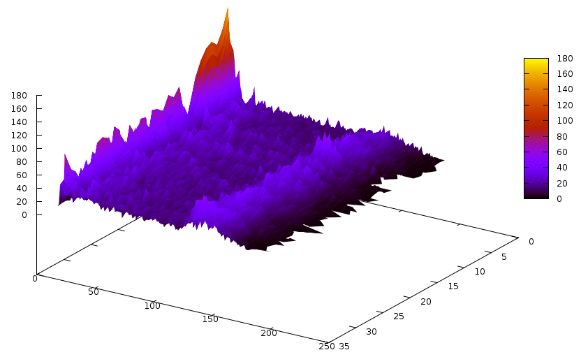
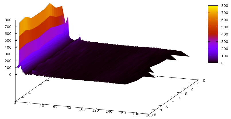
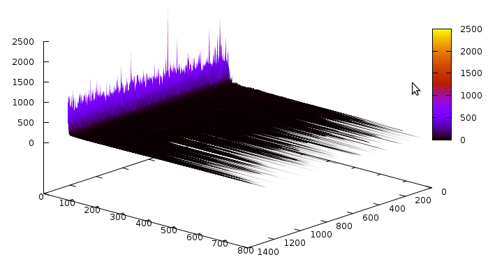
Let’s first start with the Grain cipher — we have seen it before and it had quite a peculiar shape. The learnt clause size distribution for this cipher is the following:

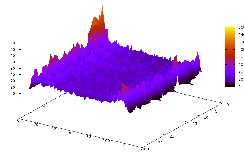
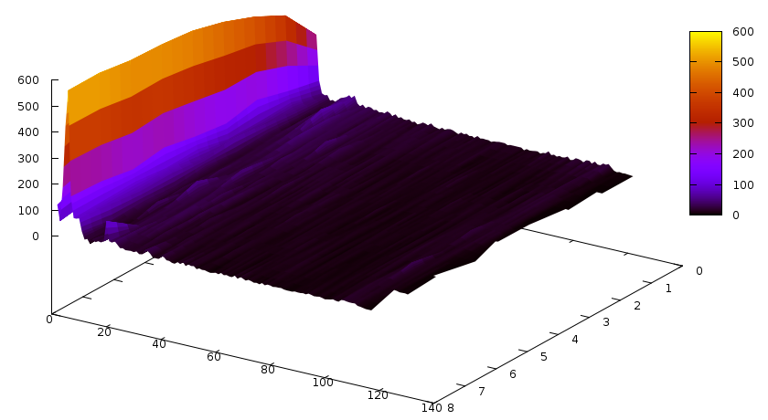
The Z axis contains the slices– one slice is 3’000 conflicts, and time flows from the back to the front (we didn’t solve the instance).The Y axis is number of clauses, and X axis is the size of the clause. Notice the bump around clause size ~130. An interesting graph would now be to compare this with glues of these clauses… so it goes:

Pretty similar, actually, except that the bump is around 110. Now, this bump could be fully useless. Or the holy grail. We don’t know… until we see some graphs ;) The graph for propagations caused by learnt clauses of specific sizes is the following:

The Z axis here is a bit different: it accumulates 3’000 propagations caused by learnt clauses, and then generates a slice. That’s the reason there are 600 of them in contrast to the one above, where there are 33 (for ~100’000 conflicts). Notice that most of the propagations are caused by small clauses. The same for glues:

Now the number of conflicts caused by learnt clauses of specific sizes:

Notice the slight colourchange on this graph at around 130 — compared to the previous 2 graphs, conflicts are done by a relatively good number of longer clauses, too. Let’s do the same with glues now:

Colourchange (and a bit visible bump, too) at around 110. Actually, it might be best to put the Y axis into logscale… next time.

ACG-20-10p0

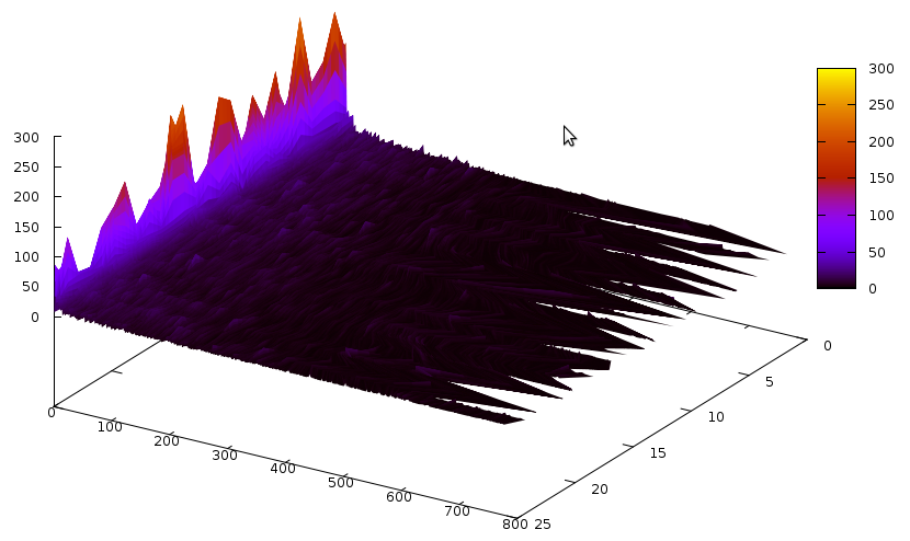
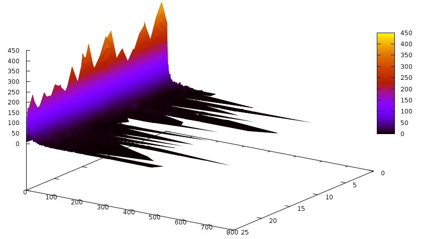
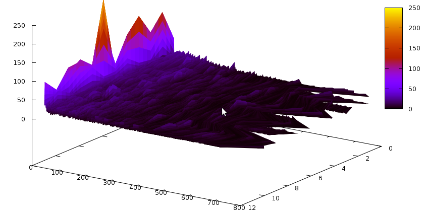
Now that we have gone through Grain, let’s try another problem. For example the ACG-20-10p0 problem from SAT Comp’09. The clause size distributions are now:

And the same for glues:

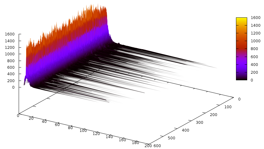
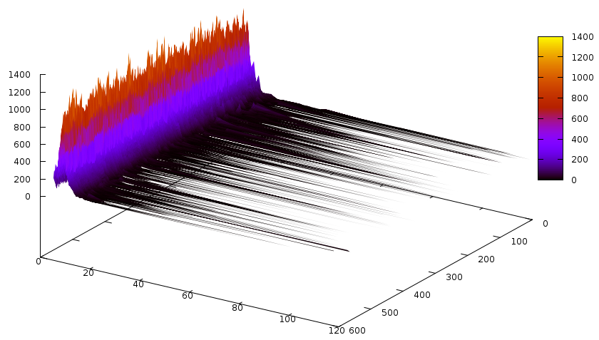
And the propagations according to their size:

Notice that the number of slices is quite large. Now the conflicts caused by learnt clauses, according to their size:

Notice that compared to the previous graph, the distribution is shifted a lot more towards longer clauses, similarly to the Grain example. Also notice that there were 25 slices in total, and 12 slices’ worth of conflicts were caused by learnt clauses — in other words, about 50% of all conflicts are caused by learnt clauses. I was aware of this behaviour because CryptoMS 1.0 had a statistical interface, where this was quite obvious to see — unfortunately, that statistical interface is gone now, but may be back in one form or another in CryptoMS 3.0.0. For Grain, we had 33 slices, and 8 slices’ worth were caused by learnt clauses, which is not 50% but still pretty high, considering that the number of learnt clauses is usually far less than the number of original clauses.

A lot of thanks go to Vegard Nossum for all of this. He was the one who inquired about producing these using the new CryptoMiniSat, and once I put the ~5 lines of code into the solver and wrote a hackish awk script, he wrote the perl script to parse the data up, and showed me the beautiful results. I just couldn’t wait to share them with you :)

Fun facts about SAT solving (part 1)

Last time I gave a talk, I got some quite deserved fire about the way I approach SAT solving: in a more practical than scientific way. So, to give some food for thought for those who wish to approach SAT from a more scientific viewpoint, and to demonstrate to what lengths I have gone to give (at least to myself) a scientific viewpoint, let me talk a little bit about a fun fact that I have found. The fun fact, as is quite usual for SAT, seems entirely trivial, even banal, but has somehow (so far) eluded proper explanation for me. Maybe you will be the one to give the right explanation :)

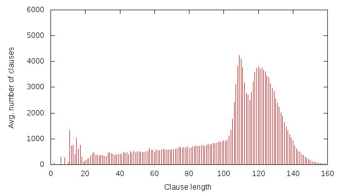
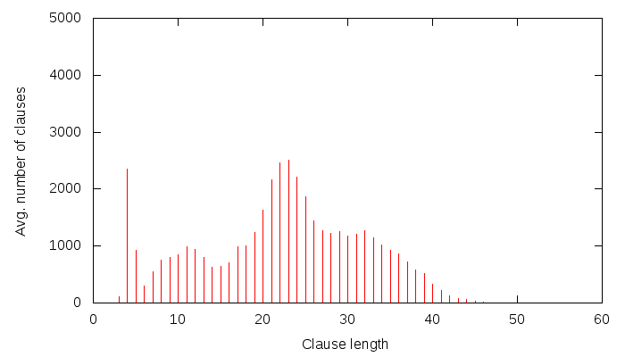
So, I generate a Grain cipher instance using, e.g. the Grain-of-Salt tool that I developed. If you don’t want to generate these yourself, there are a couple (multi-hundred thousand) pre-generated such problems you can download from here. I launch MiniSat 2.1 “core”(i.e. the most simple version) on these problems with a little twist: I write to a file the length of each generated learnt clause. Now, there are two kinds of CNF files I use: one that has 60 randomly picked randomly set state variables, and another one that is plain, and doesn’t have any variables set. Obviously, the CNF that has variables set should be easier to solve, and if Grain is a proper cipher, it should be about 2^60 easer to solve. Now, I print the average learnt clause length that I observe for the CNF that has 0 variables set, and I get this graph:

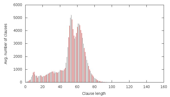
I am sure one could sing long and elaborate songs about this graph, but instead, I will just say: it has a strange curvy thing at around clause length 120. Now, I will generate a similar graph, but this time, I will use a CNF that has 60 state (i.e. important) variables set. Note that this should indeed be 2^60 times easier to solve (since Grain is a nice cipher, and my CNF generation abilities aren’t that poor). So the same graph for this CNF looks like this:

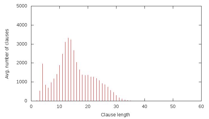
All right. This one, as I am sure you have noticed, has a curvy thing at around 60. Using elementary math, 120-60 = 60. Right, so one could reason: well, there were X unknowns, I have set 60 of them, now there are only X-60 left, so the average clause length should be 60 less! That I think doesn’t explain much, if anything, however. First off, the number of unknowns were in fact 160 — that’s the unknown state of Grain that we were trying to solve. Second, the learnt clauses don’t only contain state variables… in fact, a lot of variables they contain are not state variables at all! Furthermore, why should the 1st UIP scheme be so exact about clause sizes? After all, it’s just a graph-analysis algorithm working at the local conflict — it has no clue about the problem it is working with, much less about the number of state bits set in our instance of Grain.

One could say that this is just a dumb example, and it has no real meaning. Maybe I just stumbled upon it, after all, 120/2 = 60, etc. However, this doesn’t seem to be the case. I can, in fact, reproduce this for a lot of X’s for any of the following ciphers: Grain, Trivium, Bivium, HiTag2 and Crypto-1. Let me show one from HiTag2. Again, we are solving for the state, and we don’t set any state bits (i.e. this is the full HiTag2 problem):

Okay, there is a bumpy thing at around 23. Now, let’s set 10 randomly picked state variables to random values, and run the example again:

There seems to be a bumpy thing at around 13. 23-10 = 13. That’s about right.

By the way, I have stumbled upon the above fun fact about 2 years ago (well before CryptoMiniSat was born), when working on my diploma thesis — these graphs are actually taken verbatim from my thesis. I have worked a lot on SAT in the past 2 years, but this has been haunting me ever since. Maybe someone could explain it to me?

PS: Does anyone know if someone has done an in-depth analysis of learnt clause length distributions, maybe even three-dimensional, showing the time on the Z axis? It would be awesome to do that, if it hasn’t been done yet!

CryptoMiniSat won two gold medals at SAT Comp’11

(Note: the judges made a small mistake, and CryptoMiniSat only won 1 gold and 1 silver medal. Details below.)

CryptoMiniSat‘s SAT Competition’11 version, “Strange Night” won two gold medals at the competition: one shared with lingeling at the parallel SAT+UNSAT Applications track, and one at the parallel UNSAT Applications track. This is a great result, and I would like to thank everyone who helped me and the solver achieve this result: my fiancée, my current employer, Security Research Labs and Karsten Nohl in particular, who started the whole CryptoMiniSat saga, my former employer, INRIA Rhone-Alpes and in particular Claude Castelluccia, and finally, all the kind people at the development mailing list. Without the help of all these people, CryptoMiniSat would probably never exist in the first place, much less win such distinguished awards.

The competition was very though this year, and so it is particularly good that we have managed to win two gold medals. The most gold medals were won by the portifolio solver ppfolio, winning 5 gold medals — all other solvers won at most 2 gold medals. CryptoMiniSat did very well in the parallel applications track, basically winning all gold medals that ppfolio didn’t win — and ppfolio was using an older version of CryptoMiniSat as one of its internal engines, essentially making CryptoMiniSat compete with itself (and other strong solvers such as lingeling and clasp). Unfortunately, CryptoMiniSat didn’t win any awards at the sequential applications track, as most awards there were won by very new solvers such as Glucose ver 2 and GlueMiniSat. The source code and PDF description of these solvers are not yet available, but they will be shortly at the SAT Competition website.

Overall, I think CryptoMiniSat did very well, considering that I was not very optimistic given the fact that I didn’t manage to finish the new generation (3.x) of the solver, and had to submit a variant of the very old CryptoMiniSat 2.7.0. Furthermore, in the past year I have been concentrating on ideas external to the clause learning of SAT solvers, and it seems that the best way to speed up SAT solvers is to attack the core of the solver: the learning engine. So, this year will be about cleaning up all the external ideas and implementing new ones into the core of the solver.

Once again, thanks to everyone who helped CryptoMiniSat get such high rankings, and I am looking forward to the next year for a similarly good competition!

Edited to add (29/06):  The judges just informed me that they made a mistake, and the originally presented results were erroneous. CryptoMiniSat won 1 gold and 1 siver, as lingeling was faster by about 7% in speed in the parallel SAT+UNSAT track. Congratulations to Armin Biere for winning this track!

Dreaming up a parallel SAT architecture

When someone looks at the speed of solving when using parallel SAT solvers, it is easy to see that scaling doesn’t really work — especially for the hard UNSAT problems. In the past months I have been struggling to think of an architecture that will enable me to write a SAT solver that solves this problem. Let me share with you where I got. It will be more of a brainstorming than a descriptive blog post, but maybe it will help you avoid pitfalls, or maybe just to get a better picture of parallel SAT solving.

The constraints:

  • Clauses must be shared… all the time. Not “when it’s good enough” as per ManySat — that architecture doesn’t work well for UNSAT problems. The performance of a fully shared scheme should be able to overtake a ManySat-like architecture with ease. Only sharing low-glue or high-activity clauses does not work. This is easy to test: write a single-threaded SAT solver with high-glue learnt clause detaching on backtracking. It will work decidedly worse, even though you would clean those clauses anyway when doing clause cleaning. The reason? I don’t know… probably we need those clauses in our current local (=var activities similar) search.
  • Clauses need to have glues and activities. Glues could be dynamically updated, but the gain is not that much and the burden is a bit too much — so make that static. Activities (which are inherently dynamic) are important though (see CryptoMiniSat), and they must be lock-free as they would need to be updated frequently.
  • Memory is scarce when implication caching is used. Implication cache must be shared and updated across the parallel solvers. This not only lowers memory usage, but is an important way to share information other than clauses.
  • Parallel solvers must be lean otherwise the burden of programming a correct solver would be far too much
  • Simplifications must be carried out regularly, which needs the coordinated stopping / interruption of all parallel solvers

My architectural solution:

  • Make a lean class that only handles: clause attachment, detachment and propagation. I will need to add on-the-fly hyper-binary resolution and on-the-fly useless binary clause removal as well, as those are tightly coupled to propagation
  • Make a class that handles search&conflict generation. This class has the lean class as parent. This generates conflict clauses and has its own variable & clause activities. The class checks for new conflict clauses form other solvers after every conflict it generates, and attaches those clauses when that doesn’t need trail-rewriting — though this latter could be made optional. This class does not store a list of clauses. The tricky part of this class is on-the-fly subsumption. We will handle that by not shortening the clause but instead adding a new one and detaching the old one. The thread-coordindating class will handle the propagation of this update to all other threads. Checks for interruption are done after every generated conflict.
  • A thread-coordinating class that handles clause storage, clause distribution, and simplification. This class stops all threads if UNSAT or SAT is found by one thread, and interrupts them if clause-cleaning needs to be carried out. This class also has the lean class as parent, since e.g. clause vivification or variable-replacement need propagation.

Data structures:

  • Fully shared clauses. No move-to-front strategy, instead literal-sorting is carried out once in a while (during simplification I would assume). This has already been implemented, and is only about 10% slower than non-shared clauses in single-threaded mode.
  • Interrupt handler. This is just a flag set by the coordinating solver. The subsolvers check this flag after every conflict generated, and either exit (if SAT/UNSAT is found) or just stop and mark each learnt clause locked (if cleaning the learnt clause database)
  • Implication cache. Needs read-write lock, as most of the time it will be read to do on-the-fly self-subsuming resolution with non-existent binary clauses. Can only have literals added, not removed. Removal and updating of literals is performed only during simplification. Updating (i.e. writing) is done by threads only when doing propagation at decision level 1.
  • Distribution of newly learnt clauses. A ‘lock-free’ (how I don’t like this — it’s misleading, it has locks) datastructure for each thread in the thread-coordinating class that allows the storage of a pre-fixed number of clauses, accessible & writeable without locks until the buffer is filled (at which point we lock & update pointers).

Dilemmas:

  • Maybe thread-management while searching (i.e. learnt clause cleaning and sharing) should be a different class from the one that performs simplification. The former would not need to have propagation at all. Separation of duties always leads to cleaner code.
  • Single-threaded solving is now only an afterthought, and it would be interesting to see how the solver performs in single-threaded mode. I hope it will be only slightly worse than if it didn’t have this architecture around it. It is interesting to note, though, that the structure of the solver will be much cleaner than huge-blob single-threaded solvers tend to be.
  • OpenMP will probably not suffice, as read-write locks are not available, and implication cache sharing is a very important part of the architecture. Fully locking that datastructure when using it would incur too much overhead — most (99.9%) of the time we will be reading it. This means the code might not be as portable as I wished it would be. I think the read-write lock is the only thing I am missing to implement all of this using OpenMP.

Notes:

  • This architecture lets the designer easily change the propagation mechanism. Just re-write the lean class. I have actually done that, and I can have both move-to-front (does not work with sharing) and static clause propagation strategies. People could write their own with ease.
  • Conflict generation&search class should have an object pointer passed to it that is an instance of a class that has a abstract search class as its parent. We could then change restart settings on-the-fly by passing different object pointers.
  • We could save state (i.e. stop&restart search) easily by interrupting all threads and saving the clause database (+learnt clause cleaning state). Simplifications should be fully stateless, so no state would need to be saved for those.

Okay, this is as far as I got. I have the lean class and the search&conflict generation class, the shared clause architecture, and the stateless simplifications ready, but the coordinating class is currently highly entangled with the conflict generation class, so those need to be separated. Further, I want to fix on-the-fly subsumption because it seems to be an easy way to improve the efficiency of conflict generation: if we can shorten a non-learnt clause at every 10th conflict, that is essentially a surely good conflict clause that will never be cleaned. The effect of not having to clear clauses is important when e.g. 6x more conflicts (for a 6-core CPU) are being generated per second than with a single-threaded solver.

Understanding Implication Graphs

Having won the SAT Race with CryptoMiniSat, I think I can now confess that I still don’t understand conflict generation. So today, I sat down and I tried to understand it. The result is some fun code, a lot of reading, and great pictures. Let me share with you these auto-generated graphs — the generator will be released with CMSat 3.0.0, so you will be able to generate them, too. These graphs show something called an ‘implication graph’, which is nothing more than a graphical way to show how propagations were made by the reasoning engine. For instance, if variable x1 and x2 are both FALSE, then clause ‘x1 V x2 V x3’ will force x3 to be TRUE to satisfy the clause. Okay, so much for talk, let’s see the graphs!

Our first implication graph had a clause “-70 55 42” (light green box) that caused a conflict — that is to say, somehow the variable setting {x70=TRUE, x55=FALSE, x42=FALSE} was set, the SAT solver realised that this is wrong, and something has to be done. Let’s look at what lead here! Guesses are coloured orange here, so it seems we made the following guesses during our SAT solving: x71=TRUE, x73 = FALSE, x42=FALSE. Now, we could just say, oh, well, setting x73 to FALSE was a dumb idea, just reverse that guess, and be done with it. That’s the easy (and the fast) way, but we are less lazy than that and we want to understand the reasons. So we do something called the conflict analysis to find something called an asserting clause that will not only let us reverse the guess x73=FALSE, but will also give the SAT solver a reason why that is a necessary assignment given its previous guesses and their consequences.

Consequences in the graph are coloured dark green, and there are exactly 3 of them: x70=TRUE, x55=FALSE and x56=TRUE. Each of these is a consequence of a clause that is in the SAT solver, marked on the edge(s) leading to it. For example, x56 is set to TRUE, because of the guess x73=FALSE and the clause “x56 V x73” marked on the edge leading to x56. A consequence that has one edge leading to it was propagated by a 2-long clause, a consequence that has 2 edges leading to it was propagated by a 3-long clause (e.g. consequence “x70=TRUE”, propagated by “x70 V x55 V x73”), etc. Okay, so how do we get to the reason? Well, we start out with the conflict, the clause “-x70 V x55 V x42” (at the bottom), and we do resolutions with this clause, going bottom up. We do as many resolutions as needed to reach the first UIP (also called “articulation vertex” or “dominator”), which is a unique point on the graph through which all paths go through from the highest decision level guess, in this case x73=FALSE, at decision level 56 (noted with a @56). If you take a look, the paths from x73=FALSE diverge from the very first point onwards, and there is no single point where they converge again. This means that the (first and only) dominator will be x73=FALSE itself, and we have to resolve with all clauses on the path:

  1. Start with clause “-x70 V x55 V x42”
  2. Resolve with clause “x70 V x55 V x73”
  3. Resolve with clause “-x55 V-x56 V -x71”
  4. Resolve with clause “x56 V x73”

This list is noted on the bottommost box’s lowest entry. When we resolve with these clauses, we are actually doing cuts on the graph, like this:

My drawing capabilities aren’t exactly great, but you can see that the cuts are successively higher and higher, until we reach the cut that has on its outer part the literals -x73, x71 and -x42. Unsurprisingly, exactly the inverse of these literals are what make up the final conflict clause. Now, if we unroll the implications until decision level 47 (but not the guess x42=FALSE), then with this clause added, variable x73 will propagate to TRUE automatically, essentially reversing the wrong guess — but also giving a reason why it needs to be reversed.

If you enjoyed the previous graph, here is another to entertain you further:

And its corresponding, not too obvious solution:

Note that I was too lazy to draw cuts 10, 11 and 12 around the assignment x145=FALSE (at decision level 39). The UIP in this case is again at the decision variable, x164. If you are still interested, here are some other examples:

PS: Thanks to George Katsirelos for his help understanding this (disclaimer: all faults belong to me alone).