Note: the work below has been done in collaboration with Vegard Nossum, but the wording and some of the (mis-)conculsions are mine. If you are interested, check out his master thesis, it’s quite incredible
Anyone who has ever tried to really understand clause glues in SAT solvers have probably wondered what they really mean. Their definition is simple: the number of variables in the final conflict clause that come from different decision levels. An explanation of these terms can be found here. On the surface, this sounds very simple and clean: the number of different decision levels should somehow be connected to the number of variables that need to be set before the learnt clause activates itself, i.e. it causes a propagation or a conflict. Unfortunately, this is just the surface, because if you try to draw 2-3 implication graphs, you will see that in fact the gap between the number of variables needed to be set (let’s call this ‘activation number’) and the glue can be virtually anything, making the glue a potentially bad indicator of the activation number.
The original reasoning
The original reasoning behind glues is the following: variables in the same decision level, called ‘blocks of variables’ have a chance to be linked together through direct dependencies, and these dependencies should be expressed somehow in order to reduce the number of decisions needed to reach a conflict (and thus ultimately reduce the search space). To me, this reasoning is less clear than the one above. In fact, there are about as many intuitions about glues as the number of people I have met.
Glucosetrack
With Vegard Nossum we have developed (in exactly one day) something quite fun. On the face of it, it’s just glucose 1.0, plain and simple. However, it has an option, “-track”, which does the following: whenever a learnt clause is about to cause a conflict, it jumps over this learnt clause, saves the state of the solver, and works on until the next conflict in order to measure the amount of work the SAT solver would have had to do if that particular learnt clause had not been there. Then, when the next clause wishes to cause a conflict, it records the amount of propagation and decisions between the original conflict and this new conflict, resets the state to the place saved, and continues on its journey as if nothing had happened. The fun part here is that the state is completely reset, meaning that the solver behaves exactly as glucose, but at the same time it records how much search that particular cause has saved. This is very advantageous because it doesn’t give some magical number like glue, but actually measures the usefulness of the given clause. Here is a typical output:
c This is glucose 1.0  with usefulness tracking by
c Vegard Nossum and Mate Soos. Based on glucose, which
c is in run based on MiniSat, Many thanks to all teams
c
c ============================[ Problem Statistics ]=============================
c |                                                                             |
c |  Number of variables:  138309                                               |
c |  Number of clauses:    942285                                               |
c |  Parsing time:         0.28         s                                       |
============================[ Search Statistics ]==============================
| Conflicts |          ORIGINAL         |          LEARNT          | Progress |
|           |    Vars  Clauses Literals |    Limit  Clauses Lit/Cl |          |
===============================================================================
|         0 |  138309   942285  2636352 |   314095        0   -nan |  0.000 % |
|       620 |  138074   942285  2636352 |   314095      615     82 |  1.559 % |
|       919 |  135307   925938  2596895 |   314095      906     75 |  3.908 % |
|      2714 |  130594   894562  2518954 |   314095     2664     67 |  6.799 % |
|      2814 |  130593   894562  2518954 |   314095     2763     69 |  6.808 % |
|      2930 |  130592   894562  2518954 |   314095     2879     70 |  6.808 % |
|      4042 |  127772   874934  2471045 |   314095     3974     69 |  9.292 % |
|      4142 |  127772   874934  2471045 |   314095     4074     70 |  9.292 % |
...
c Cleaning clauses (clean number 0). Current Clause usefulness stats:
INSERT INTO data(cleanno, idx, size, glue, conflicts, props, bogoprops, decisions) VALUES(0 , 961074 , 107 , 5 , 42 , 185509 , 1301341 , 0);
INSERT INTO data(cleanno, idx, size, glue, conflicts, props, bogoprops, decisions) VALUES(0 , 944729 , 14 , 1 , 7 , 36865 , 268229 , 0);
INSERT INTO data(cleanno, idx, size, glue, conflicts, props, bogoprops, decisions) VALUES(0 , 948275 , 7 , 1 , 15 , 27909 , 220837 , 0);
INSERT INTO data(cleanno, idx, size, glue, conflicts, props, bogoprops, decisions) VALUES(0 , 953762 , 102 , 2 , 2 , 29365 , 197410 , 0);
...
c End of this round of database cleaning
...
|     38778 |  110896   758105  2182915 |   314095    28270     93 | 20.167 % |
|     39488 |  110894   758105  2182915 |   314095    28978     93 | 20.185 % |
c Cleaning clauses (clean number 1). Current Clause usefulness stats:
INSERT INTO data(cleanno, idx, size, glue, conflicts, props, bogoprops, decisions) VALUES(1 , 979236 , 71 , 1 , 8 , 45531 , 280156 , 0);
INSERT INTO data(cleanno, idx, size, glue, conflicts, props, bogoprops, decisions) VALUES(1 , 954908 , 2 , 2 , 7 , 0 , 232760 , 0);
...
The output is in SQL format for easy SQL import. The “size” is the clause size, “glue” is the glue number, “conflicts” is the number of times the clause caused a conflict, “props” is the number of propagations gained by having that clause (i.e. by doing the conflict early), “bogoprops” is an approximation of the amount of time gained based on the number of watchlists and the type of clauses visited during propagation, and “decisions” is the number of decisions gained. The list is sorted according to “bogoprops”, though once the output is imported to MySQL, many sortings are possible. You might notice that the ‘glue’ is 1 for some clauses (e.g. on the second output line) — these are clauses that have caused a propagation at decision level 0, so they will eventually be removed through clause-cleaning, since they are satisfied. Notice that high up, there are some relatively large clauses (of size 102 for example) with glue 2, that gain quite a lot in terms of time of search. The gained conflicts/propagations/etc. are all cleared after every clause-cleaning, though since clauses are uniquely indexed (‘idx’), they can be accumulated in all sorts of ways.
The program is 2-5x slower than normal glucose, but considering that it has to save an extreme amount of state due to the watchlists being so difficult to handle and clauses changing all the time, I think it does the job quite well — as a research tool it’s certainly quite usable. In case you wish to download it, it’s up in GIT here, and you can download a source tarball here. To build, issue “cmake .” and “make”. Note that the tool only measures the amount of search saved by having the clause around when it tries to conflict. It does not measure the usefulness of the propagations that a learnt clause makes. Also, it doesn’t measure the other side of the coin: the (potentially better) conflict generated by using this clause instead of the other one. In other words, it gives a one-sided view (no measure of help through propagation) of a one-sided view (doesn’t measure the quality of difference between the conflict clauses generated). Oh well, it was a one-day hack.
Experiments
I have made very few experiments with glucosetrack, but you might be interested in the following result. I have taken UTI-20-10p0, ran it until completion, imported the output into MySQL, and executed the following two queries. The first one:
SELECT glue, AVG(props), FROM data
WHERE glue >= 2 AND size >= 2
GROUP BY glue
ORDER BY glue
calculates the average number of saved propagations between each round of cleaning for clauses of glue >= 2 (i.e. clauses that didn’t eventually cause a propagation at decision level 0), and of size >= 2, because unitary clauses are of no interest. The second is very similar:
SELECT size, AVG(props), FROM data
WHERE glue >= 2 AND size >= 2
GROUP BY size
ORDER BY size
which calculates the same as above, but for size.
Some explanation is in order here regarding why I didn’t count SUM(), and instead opted for AVG(). In fact I personally did make graphs for SUM(), but Vegard corrected me: there is in fact no point in doing that. If I came up with a new glue calculation function that gave an output of ‘1’ for every clause, then the SUM for that function would look perfect: every clause would be in the same bracket, saving a lot of propagations, but that would not help me make a choice of which clauses to throw out. But the point of glues is exactly that: to help me decide which clauses to throw out. So what we really want is a usefulness metric that tells me that if I keep clauses in that bracket, how much do I gain per clause. The AVG() gives me that.
Here goes the AVG() graph for the last clause cleaning (clause cleaning iteration 33):
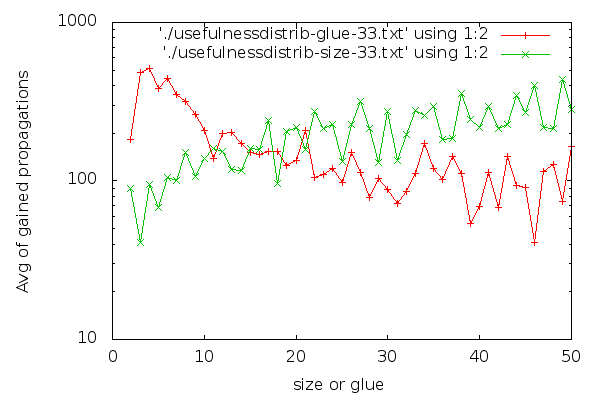
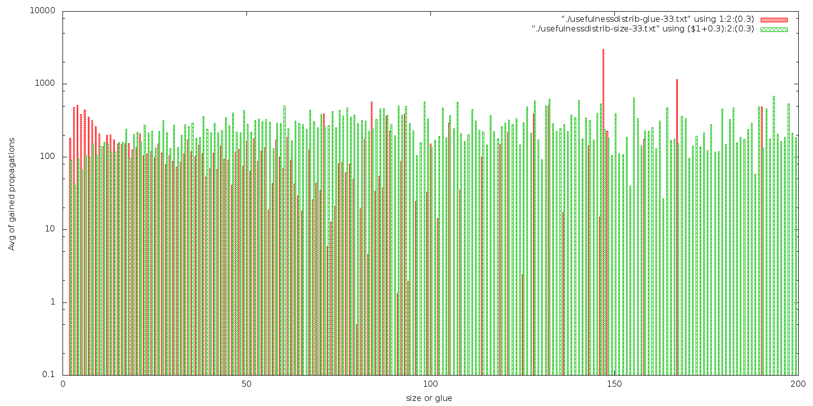
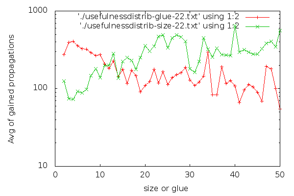
Notice that the y axis is in logscale. In case you are interested in a larger graph, here it is. The graph for clause cleaning iteration 22 is:
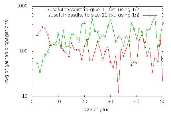
 (Iteration 11 has high fluctuations due to less data, but for the interested, here it is). I think it’s visible that glues are good distinguishers. The graph for glues drops down early and stays low. For sizes, the graph is harder to read. Strangely, short clauses are not that good, and longer clauses are better on average. If I had to make a choice about which clauses to keep based on the size graph, it would be a hard choice to make: I would be having trouble selecting a group that is clearly better than the rest. There are no odd-one-out groups. On the other hand, it’s easier to characterise which clauses are good to have in terms of glues: take the low glue ones, preferably below 10, though we can skip the very low ones if we are really picky. An interesting side-effect of the inverse inclination of the size and glue graphs and the fact that “glue<=size” is that maybe we could choose better clauses to keep if we go for larger clauses that have a low glue.
Conclusions
Unfortunately, there are no real conclusions to this post. I guess running glucosetrack for far more than just one example, and somehow also making it measure the difference between the final conflict clauses’ effectiveness would help to write some partially useful conclusion. Vegard and me have tried to put some time and effort into this, but to not much avail I am afraid.
PS: Notice that glucosetrack allows you to generate many of the graphs here using the right SQL query.