I have recently had a few discussions with people who wanted to do some form of model counting, and I decided to put my thoughts about this problem into a single blog post, hopefully bringing some light to this area. Firstly, when talking about model counting, it’s very important to think through what one actually needs to achieve. When people talk about a model, they often mean a solution to a problem, described as a set of constraints over either purely boolean variables (so-called propositional model counting) expressed in so-called CNF, or over higher-level constraints, often expressed in SMT-LIB format.
Let’s look at a CNF example:
c this is a comment
c below line means there are 5 boolean variables and 2 constraints
p cnf 5 2
1 -2 0
1 -2 3 0
The above CNF has 5 boolean variables and 2 constraints: “v1 or (not v2) = true”, and “v1 or (not v2) or v3 = true”. In this case, if “v1 or (not v2) = true” is satisfied, the other constraint is also satisfied. So we effectively only have to satisfy the “v1 or -v2” constraint. There are 3 solutions over the variables v1 and v2 to this constraint: (1, 0), (1, 1), and (0,0). For variables v3, v4, and v5 we can choose anything. So there are a total of 3*2^3 = 24 solutions to this CNF.
Let’s look at an SMT problem:
(set-logic QF_BV) ; Set the logic to Quantifier-Free BitVectors
(declare-fun bv () (_ BitVec 8)) ; Declare an 8-bit value
(assert (not (= bv #x00))) ; Assert that 'bv' is not equal to zero
In this SMT-LIB problem, we declared that the logic we will be using is the so-called quantifier-free bitvector logic, which basically gives you access to fixed-width variables such as uint8_t, and of course all the logical and fixed-bit bitwector operators such as modulo addition, division, subtraction, etc. In this particular case, we declared an 8-bit variable and banned it from being 0, so this problem has 2^8-1 solutions, i.e. 255.
Whichever format is being used, “counting” of solutions is something that may sound trivial (it’s just a number!), but once we get a bit more fiddly, it turns out that we can do many things that are actually easier, or even harder, than just counting, even though they sound very close to, or are even synonymous with, counting :
- Figuring out if there is at least one solution. This is more appropriately called satisfiability checking. This is significantly easier than any notion of counting listed below. However, even this can be challenging. Typically, in the SMT/SAT competition, this is the so-called SMT single query track or the SAT competition Main Track. All SAT and SMT solvers such as kissat or cvc5 can run this kind of task.
- Next up in complexity is to figure out if there is exactly one solution. This is actually very close to satisfiability checking, and requires only two so-called “incremental calls” to the SMT/SAT solver. I have seen this question pop up a lot in zero-knowledge (ZK) circuit correctness. What is needed is to run the query as per the above, but then add a constraint that bans the solution that is output by the solver, and ask the system to be solved again. If the solver outputs UNSAT, i.e. unsatisfiable, then we know there are no more solutions, and we are happy with the result. If not, it gives us another solution, which is a witness that there are at least two solutions. These queries are answered by so-called incremental SMT solvers (SMT competition track here), or incremental SAT solvers (incremental SAT competition track here). Almost all SAT and SMT solvers can work incrementally, for example cvc5 or z3. Most SAT solvers work incrementally, too, but e.g. kissat does not, and you need to use CaDiCaL instead.
- Next up in complexity is to approximately count the solutions. Here, we are not interested that there are exactly, say, 87231214 solutions, instead, we are happy to know that there are approx 2^26 solutions. This is often good enough, in case one wants to e.g. figure out probabilities. There are very few such systems available, for SMT there is csb, and for SAT there is ApproxMC. For the special case of approximate DNF counting, I’d recommend pepin.
- Next up in the complexity is exactly counting the solutions. Here, we want to know how many solutions there are, exactly, and we really-really need the exact number. There are few solutions to doing this over SMT, but doing this over SAT is quite developed. For SMT, I would recommend following the csb approach, and running Ganak on the blasted SAT formula instead of ApproxMC, and for SAT, there is the annual model counting competition, where Ganak won every single category this year, so I’d recommend Ganak.
- Next up is model enumeration where it’s not enough to count the solutions, but we need a way to compactly represent and store them all. This of course requires quite a bit of disk space, as there could be e.g. 2^100 solutions, and representing them all, even in a very compact format with lots of smart ideas can take a lot of space — but not necessarily exponential amount. Currently, there is no such system for SMT, and my understanding is that only the d4 model counter can do this on SAT/CNF problems, thanks to its proof checking system, in part thanks to Randal Byrant. Once Ganak can output a proof, it will also be able to do this.
All in all, there is a very large gap between “find if there is exactly one solution” and “enumerate all solutions” — even though I have seen these two notions being mixed up a few times. The first might take only a few seconds to solve, while the other might not even be feasible, because compactly representing all solutions may be too expensive in terms of space (and that’s not even discussing time).
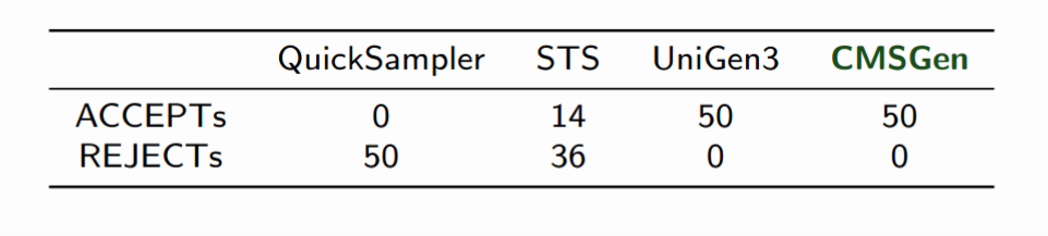
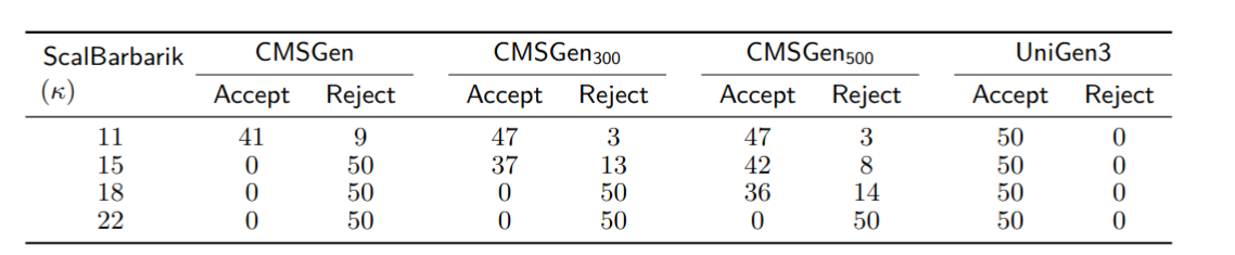
One aspect to keep in mind is that often, one does not need all solutions. For example, if one only wants to find a good set of example solutions, then it is possible to use uniform-like samplers, that give a “somewhat uniform” set of example solutions from the solution space (without guarantees of uniformity). A good tool for this is cmsgen for CNF/SAT problems. If one needs a guaranteed uniform set of samples (to be exact, a probabilistically approximately uniform sample), then unigen is the way to go. Obviously, it’s quite easy to find a uniform sample once we have an enumeration of all solutions — simply pick a random one from the whole set — but that’s way more expensive than running unigen.
While all of the above is about counting, it’s often the case that one wants to optimize for something within the solution space. Basically, we have some kind of objective function that we want to optimize for (e.g. maximize profit, minimize loss) , and so we are looking for a solution that maximizes/minimizes some property. Of course, once we have done model enumeration, it’s quite easy to do this — simply run the objective function on all solutions, and pick the best! But that’s really hard. Instead, one can formulate the problem as a so-called MaxSAT or an SMT problem with an objective function. These systems run some really smart algorithms to significantly cut down search time, and even often keep a “best so far” solution around, so we can early-abort them and still get some kind of “best so far” solution.
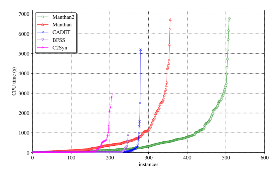
All in all, it’s extremely important to figure out what one actually needs, because there are vast gaps in complexity between the problems (and corresponding algorithms) above. Even between something like approximate and exact counting, the gap is gigantic, as there are huge swaths of problems that are almost trivial to count approximately, but essentially impossible to exactly count with current technology:

Here, the green line is a tool that changes its behaviour from exact to approximate model counting after 1800 seconds of solving, and the number of solved instances jumps significantly. Notice that the red line, the original system it runs for 1800s, is the best in class here, by a wide margin, and still the approximate counting that Ganak+ApprocMC switches into shows a massive difference.