Category Archives: Research

Research-related information

ApproxMCv3, a modern approximate model counter

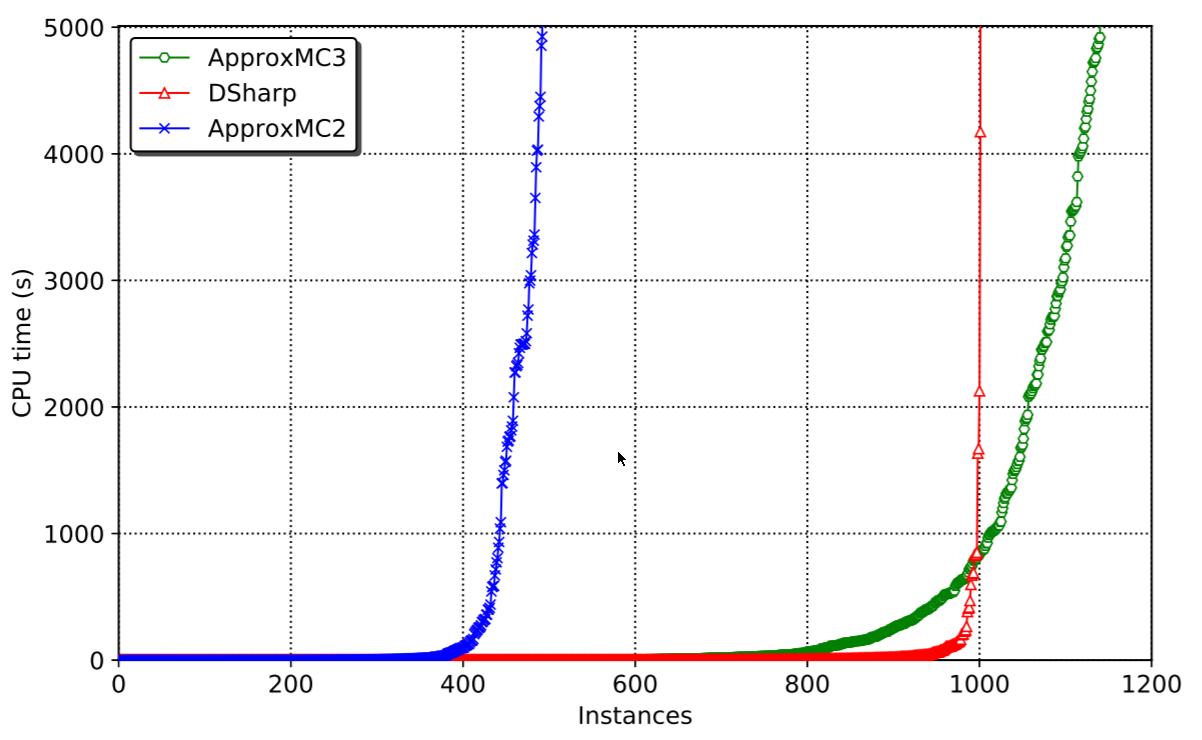
This blogpost and its underlying work has been brewing for many years, and I’m extremely happy to be able to share it with you now. Kuldeep Meel and myself have been working very hard on speeding up approximate model counting for SAT and I think we have made real progress. The research paper, accepted at AAAI-19 is available here. The code is available here (release with static binary here). The main result is that we can solve a lot more problems than before. The speed of solving is orders(!) of magnitude faster than the previous best system:

Background

The idea of approximate model counting, originally by Chakraborty, Meel and Vardi was a huge hit back in 2013, and many papers have followed it, trying to improve its results. All of them were basically tied to CryptoMiniSat, the SAT solver that I maintain, as all of them relied on XOR constraints being added to the regular CNF of a typical SAT problem.

So it made sense to examine what CryptoMiniSat could do to improve the speed of approximate counting. This time interestingly coincided with me giving up on XORs in CryptoMiniSat. The problem was the following. A lot of new in- and preprocessing systems were being invented, mostly by Armin Biere et al, and I quickly realised that I simply couldn’t keep adding them, because they didn’t take into account XOR constraints. They handled CNF just fine, but not XORs. So XORs became a burden, and I removed them in versions 3 and 4 of CryptoMiniSat. But there was need, and Kuldeep made it very clear to me that this is an exciting area. So, they had to come back.

Blast-Inprocess-Recover-Destroy

But how to both have and not have XOR constraints? Re-inventing all the algorithms for XORs was not a viable option. The solution I came up with was a rather trivial one: forget the XORs during inprocessing and recover them after. The CNF would always remain the source of truth. Extracting all the XORs after in- and preprocessing would allow me to run the Gauss-Jordan elimination on the XORs post-recovery. So I can have the cake and eat it too.

The process is conceptually quite easy:

  1. Blast all XORs into clauses that are in the input using intermediate variables. I had all the setup for this, as I was doing Bounded Variable Addition  (also by Biere et al.) so I didn’t have to write code to “hide” these additional variables.
  2. Perform pre- or inprocessing. I actually only do inprocessing nowadays (as it has faster startup time). But preprocessing is just inprocessing at the start ;)
  3. Recover the XORs from the CNF. There were some trivial methods around. They didn’t work as well as one would have hoped, but more on that later
  4. Run the CDCL and Gauss-Jordan code at the same time.
  5. Destroy the XORs and goto 2.

This system allows for everything to be in CNF form, lifting the XORs out when necessary and then forgetting them when it’s convenient. All of these steps are rather trivial, except, as I later found out, recovery.

XOR recovery

Recovering XORs sounds like a trivial task. Let’s say we have the following clauses

 x1 V  x2 V  x3
-x1 V -x2 V  x3
 x1 V -x2 V -x3
-x1 V  x2 V -x3

This is conceptually equivalent to the XOR v1+v2+v3=1. So recovering this is trivial, and has been done before, by Heule in particular, in his PhD thesis. The issue with the above is the following: a stronger system than the above still implies the XOR, but doesn’t look the same. Let me give an example:

 x1 V  x2 V  x3
-x1 V -x2 V  x3
 x1 V -x2 V -x3
-x1 V  x2

This is almost equivalent to the previous set of clauses, but misses a literal from one of the clauses. It still implies the XOR of course. Now what? And what to do when missing literals mean that an entire clause can be missing? The algorithm to recover XORs in such cases is non-trivial. It’s non-trivial not only because of the complexity of how many combinations of missing literals and clauses there can be (it’s exponential) but because one must do this work extremely fast because SAT solvers are sensitive to time.

The algorithm that is in the paper explains all the bit-fiddling and cache-friendly data layout used along with some fun algorithms that I’m sure some people will like. We even managed to use compiler intrinsics to use target-specific assembly instructions for hamming weight calculation. It’s a blast. Take a look.

The results

The results, as shown above, speak for themselves. Problems that took thousands of seconds to solve can now be solved under 20. The reason for such incredible speedup is basically the following. CryptoMiniSatv2 was way too clunky and didn’t have all the fun stuff that CryptoMiniSatv5 has, plus the XOR handling was incorrect, loosing XORs and the like. The published algorithm solves the underlying issue and allows CNF pre- and inprocessing to happen independent of XORs, thus enabling CryptoMiniSatv5 to be used in all its glory. And CryptoMiniSatv5 is fast, as per the this year’s SAT Competition results.

Some closing words

Finally, I want to say thank you to Kuldeep Meel who got me into the National University of Singapore to do the work above and lots of other cool work, that we will hopefully publish soon. I would also like to thank the National Supercomputing Center Singapore  that allowed us to run a ton of benchmarks on their machines, using at least 200 thousand CPU hours to make this paper. This gave us the chance to debug all the weird edge-cases and get this system up to speed where it beats the best exact counters by a wide margin. Finally, thanks to all the great people I had the chance to meet and sometimes work with at NUS, it was a really nice time.

CryptoMiniSat and Parallel SAT Solving

Since CryptoMiniSat has been getting quite a number of awards with parallel SAT solving, it’s about time I talk about how it does that.There is a ton of literature on parallel SAT solving, and I unfortunately I have barely had time to read any of them. The only research within the parallel SAT solving area that I think has truly weathered the test of time is Plingeling and Treengeling — and they are really interesting to play with. The rest most likely  has some merit too, but I am usually suspect as the results are often –unintentionally — skewed to show how well the new idea performs and in the end they rarely win too many awards, especially not in the long run (this is where Plingeling and Treengeling truly shine). I personally haven’t published what I do in this scene because I have always found it to be a bit too easy and to hence have little merit for publication — but maybe one day I will.

Note: by unintentionally skewed results I mean that as you change parameters, some will inevitably be better than others because of randomness in the SAT solving. This randomness is easy to mistake for positive results. It has happened to everyone, I’m sure, including myself.

Exploiting CryptoMiniSat-specific features

CryptoMiniSat has many different inprocessing systems and many parameters to turn them on/off or to tune them. It has over 60k lines of code which allows this kind of flexibility. This is unlike the Maple*/Glucose* set of solvers, all coming from MiniSat, which basically can do one thing, and one thing only, really well. That seriously helps in the single-threaded setup, but may be an issue when it comes to multi-threading. They have (almost) no inprocessing (there is now vivification in some Maple* solvers), and no complicated preprocessing techniques other than BVE, subsumption and self-subsuming resolution. So, there is little to turn on and off, and there are very few parameters — and the few parameters that are there are all hard-coded into the solver, making them difficult to change.

CryptoMiniSat in parallel mode

To run in parallel mode, CMS takes advantage of its potential heterogeneity by running N different threads, each with radically different parameter settings, and exchanging nothing but unit and binary clauses(!) with the most rudimentary locking system. No exchange of longer clauses, no lockless exchanges, no complicated multi-lock system. One lock for unit clauses, one for binary, even for 24 threads. Is this inefficient? Yes, but it seems good enough, and I haven’t really had too many people asking for parallel performance. To illustrate, here are the parameter sets of the different threads used and here is the sharing and locking system. It’seriously simple, I suggest you take a peek, especially at the parameter sets.

Note that the literature is full of papers explaining what kind of complicated methods can be used to exchange clauses using different heuristics, with pretty graphs, complicated reasoning, etc. I have to admit that it might be useful to do that, however, just running heterogeneous solvers in parallel and exchanging unit&binary clauses performs really well. In fact, it performs so well that I never, ever, in the entire development history of 7 years of CMS, ran even one full experiment to check parallel performance. I usually concentrate on single-threaded performance because checking parallel performance is really expensive.

Checking the performance of a 24 thread setup is about 15x more expensive than the single-threaded variant. I don’t really want to burn the resources for that, as I think it’s good enough as it is. It’s mostly beating solvers with horrendously complicated systems inside them with many research papers backing them up, etc. I think the current performance is proof enough that making things complicated is not the only way to go. Maybe one day I will implement some more sophisticated clause sharing, e.g. sharing clauses that are longer than binary and then I won’t be able to claim that I am doing something quite simple. I will think about it.

Conclusions

I am kinda proud of the parallel performance of CMS as it can showcase the heterogeneity of the system and the different capabilities of the solver. It’s basically doing a form of acrobatics where the solver can behave like a very agile SAT solver with one set of parameters or like a huge monolith with another set of parameters. Since there are many different parameters, there are many different dimensions, and hence there are many orthogonal parameter sets. It’s sometimes interesting to read through the different parameter settings and wonder why one set works so much better than the other on a particular type of benchmark. Maybe there could be some value in investigating that.

CryptoMiniSat 5.6.3 Released

The latest CryptoMiniSat, version 5.6.3 has been released. This release marks the 12’000th commit to this solver that has weathered more than I originally intended it to weather. It’s been an interesting ride, and I have a lot to thank Kuldeep and NSCC‘s ASPIRE-1 cluster for this release. I have burned over 200k CPU hours to make this release, so it’s a pretty well-performing release (out-performing anything out there, by a wide margin), though I’m working very hard to make sure that neither I nor anyone else will have to burn anything close to that to make a well-performing SAT solver.

The solver has some interesting new algorithms inside, the most interesting of which is Gauss-Jordan elimination using a Simplex-like method, generously contributed by Jie-Hong Roland Jiang and Cheng-Shen Han from the National Taiwan University. This addition should finally settle the issues regarding Gaussian vs Gauss-Jordan elimination in SAT solvers. Note that to use this novel system, you must configure with “cmake -DUSE_GAUSS=ON ..” and then re-compile.

What’s also interesting is what’s not inside, though. I have been reading (maybe too much) Nassim Taleb and he is very much into via negativa. So I tried removing algorithms that have been in the solver for a while and mostly nobody would question if they are useful. In the end I removed the following algorithms from running by default, each removal leading to better solving time:

  • Regular probing. Intree probing is significantly better, so regular probing is not needed. Thanks Matti/Marijn/Armin!
  • Stamping. This was a big surprise, especially because I also had to remove caching, which is my own, crappy (“different”) version of stamping. I knew that it wasn’t always so good to have, but damn. It was a hard call, but if it’s just slowing it down, what can I do. It’s weird.
  • Burst searching. This is when I search for a short period with high randomness all over the search space. I thought it would allow me to explore the search space in places where VSIDS/Maple doesn’t. Why this is slowing the solver down so much may say more about search heuristics/variable bumping/clause bumping than anything.
  • Note that I never had blocked clause elimination. It doesn’t work well for incremental solving. In fact, it doesn’t work at all, though apparently the authors have some new work that allows it to work, super-interesting!

I’m nowadays committed to understanding this damned thing rather than adding another impossible-to-explain magic constant  to make the solving 10% faster. I think there is interesting stuff out there that could be done to make SAT solvers 10x, not 10%, faster.

Machine Learning and SAT

I have lately been digging myself into a deep hole with machine learning. While doing that it occurred to me that the SAT community has essentially been trying to imitate some of ML in a somewhat poor way. Let me explain.

CryptoMiniSat and clause cleaning strategy selection

When CryptoMiniSat won the SAT Race of 2010, it was in large part because I realized that glucose at the time was essentially unable to solve cryptographic problems. I devised a system where I could detect which problems were cryptographic. It checked the activity stability of variables and if they were more stable than a threshold, it was decided that the problem was cryptographic. Cryptographic problems were then solved using a geometric restart strategy with clause activities for learnt database cleaning. Without this hack, it would have been impossible to win the competition.
Continue reading Machine Learning and SAT

Why it’s hard to eliminate variables

Let’s examine why it’s hard to eliminate variables. I remember the code I looked at in SatElite that did it: it was crazy clean code and looked like it was pretty easy to perform. In this post I’ll examine how that simple code became more than a 1’000 lines of code today.

What needs to be done, at first sight

At first sight, variable elimination is easy. We just:

  1. Build occurrence lists
  2. Pick a variable to eliminate
  3. Resolve every clause having the positive literal of the variable with negative ones.
  4. Add newly resolved clauses into the system
  5. Remove original clauses.
  6. Goto 2.

These are all pretty simple steps at first sight, and one can imagine that implementing them is maybe 50-100 lines of code, no more. So, let’s examine them one-by-one to see how they get complicated.

Building occurrence lists

The idea is that we simply take every single clause, and for every literal they have, we insert a pointer to the clause into an array for that literal’s occurrences. This sounds easy, but what happens if we are given 1M clauses, each with 1000 literals on average? If you think this is crazy, it isn’t, and does in fact happen.

One option is we estimate the amount of memory we would use and abort early because we don’t want to run out of memory. So, first we check the potential size, then we link them in. Unfortunately, this means we can’t do variable elimination at all. Another possibility is that we link in clauses only partially. For example, we don’t link in clauses that are redundant but too long. Redundant clauses are ignored during resolution when eliminating, so this is OK, but then we will have to clean these clauses up later, when finishing up. However, if a redundant clause that hasn’t been linked in backward-subsumes an irredudant clause (and thus becomes irredundant itself), we have to link it in asap. Optimisation leads to complexity.

We don’t just want to link these clauses in to some random datastructure. I believe it was Armin Biere who put this idea into my head, or maybe someone else, but re-using watchlists for occurrence lists means we use our memory resources better: there won’t be so much fragmentation. Furthermore, an advanced SAT solver uses implicit binary & tertiary clauses, so those are linked in already into the watchlists. That saves memory.

Picking a variable to eliminate

The order in which you eliminate clauses is a defining part of the speed we get with the final solver. It is crucially important that this is done well. So, what can we do? We can either use some heuristic or precisely calculate the gain for each variable, and eliminate the best guess/calculated one first. These are both greedy algorithms but I think given the complexity of the task, they are the best at hand.

Using precise calculation is easy, we just resolve all the relevant clauses but don’t add the resolvents. It’s very expensive though. A better approach is to use a heuristic. Logically, clauses that have few literals in them are likely not to resolve such that they become tautologies. It’s unlikely that two binary clauses’ resolvent becomes a tautology. It’s however likely that large clauses become tautological once resolved. I take this into account when calculating elimination cost for variable. Since redundant clauses are linked in the occurrence lists so that I can subsume them, I have to skip them.

It’s not enough to calculate the heuristic once, of course. We have to re-calculate after every elimination — the playing field has changed. Thus, for every clause you removed, you have to keep in mind which variables were affected, and re-calculate the cost for each after every variable elimination.

Resolving clauses

The base is easy. We add literals to a new array of literls and mark the literals that have been added in a quick-lookup array. If the opposite of a literal is added, the markings tell us and we can skip the rest — the resolvent is tautological. Things get hairy if the clause is not tautological.

What if the new clause is subsumed by already-existing clauses? Should we check for this? This is called forward-subsumption, and it’s really expensive. Backward subsumption (which asks the question ‘Does this clause subsume others?’ instead of ‘Is this clause subsumed by others?’) would be cheaper, but that’s not the case here. We can thus try to subsume the clause only by e.g. binary&tertiary clauses and hope for the best.

What if the new clause can be subsumed by stamps? That’s easy to check for, but if the new clause was used to create the stamp, that would be a self-dependency loop and not adding the resolvent would lead to an incorrect result. We can use the stamps as long as the resolving clauses were not needed for the stamp: i.e. they are not binary clauses and on-the-fly hyper-binary resolution was used during every step of stamp generation. A similar logic goes for using the implication cache.

We could also virtually extend the clause with literals using watchlists/stamps/impl. cache and then try to subsume that virtual clause. I forgot what 3-letter acronym Biere et al. gave to this method (it’s one of the 12 on slide 25 here), but, except for the acronym, this idea is pretty simple. You take a binary clause, e.g. xV~y, and if x is in the newly created clause, but y and ~y is not, you add y to the clause. The clause is now bigger, so has a larger chance to be subsumed. You now perform forward subsumption as above, but with the extended clause. Also, take care not to subsume clauses with themselves, which, as you might imagine, can get hairy.

If all of this sounds a bit intricate, this is not even the difficult part. The difficult part is keeping track of time. Where of course by time I don’t actually mean seconds — I mean computation steps that you have to define one way or another and increment counters and set limits. Remember: all this has to be deterministic.

Doing all of the above with a small but complicated instance is super-fast, under 0.001s. With a weird instance where one single literal may occur in more than a million clauses, it can be very-very expensive even for one single try — over 100s. That’s about 5 orders of magnitude of difference. So, you have to be careful. The resolution we cannot skip, but we can abort it (and indicate it up in the call tree). Some of the others we can abort, but then the whole resolution has to be re-started. Some of the above is not critical at all, so you have to use a different time-limit for some, and mark them as too expensive, so at least the basic things get done. This gets complicated, because e.g. forward-subsumption you might want to re-use at other parts of the solver so you have to use a time-limit that isn’t global.

Adding the newly resolved clauses

Adding clauses is simple: we create and link them in. However, we can do more. Since backward-subsumption is fast, we can do that with the newly created clauses. Note that this means the newly created clause could subsume some of the original clauses it was created from — which means the resolvents should be pre-generated and kept in memory.

Another thing: since we know the new clause needs to be added, we might as well shorten it before in any way we can. At this point, we can make use of all the watchlists, stamps and implication cache we have to shorten the new clause: there are no problems with self-dependencies. It will pay off. However, note that shortening the clause before adding it means that we will have to reverse-shorten it later, when this clause might be part of a group of clauses that is touched by a new variable elimination round. So, we are working against ourselves in a way — especially because reverse shortening is pretty expensive and hairy as explained above.

Although this is obvious, but we still have to take care of time-outs. For example, if resolution took so much time that we are already out of time, we must exit asap and not worry about the resolvents. Don’t link, don’t remove, just exit. Time is of essence.

Removing the original clauses

Easy, just unlink them from the occurrence lists. I mean, easy if you don’t care about time, of course. Because unlinking is an O(N^2) operation if you have N clauses and all of them contain the same literal X — the N-long occurrence list of literal X has to be read and updated N times. So, we don’t do this.

First of all, a special case: the two occurrence lists of the variable we are removing can simply be .clear()-ed. It’s no longer needed. Secondly, we shouldn’t unlink clauses one-by-one. Instead, we should mark the clause as removed, and then not care about the clause later. Once variable elimination is finished, we do a sweep of all the occurrence lists and clauses and remove the clauses that have been marked. This means that e.g. forward and backward subsumption gets more hairy (we shouldn’t subsume with a clause that’s been marked as removed but is still in the occurrence list) but that O(N^2) becomes O(N) which for problems where N is large makes quite a bit of difference. Like, the difference of 100s vs. 10s for a the same exact thing.

The untold horrors

On top of what’s above, you might like to generate some statistics about what worked and what didn’t. You might like to dump these statistics to a database. You might like to not create resolutions that are not needed as the irreduntant clauses form an AND/ITE gate. Or multiple gates. You might like to eliminate only a subset of variables at each call so that you don’t make your system too sparse and thus reduce arc consistency. You might want to vary this limit based on the problem at hand. You might want to do many other things that are not detailed above.

Conclusions

Once I read through the above, I realized I kind of missed the essence: time-outs. It’s mentioned here and there, but it’s much more critical than it seems and makes things a hell of a lot harder. How do you cleanly exit from the middle of reverse-shortening while resolving because you ran out of time? I could just bury my head in sand of course and say: I don’t care. Or, I could make some messy algorithm that checks return values of each call and return a special value in case of time-outs. This needs to be done for every level of the call, which can be pretty deep, unless you like writing 1’500 line functions. I wanted to say writing&reading, but, really, nobody reads 1’500 line functions. They are throw-away,write-only code.