Tag Archives: visualisation

Understanding Implication Graphs

Having won the SAT Race with CryptoMiniSat, I think I can now confess that I still don’t understand conflict generation. So today, I sat down and I tried to understand it. The result is some fun code, a lot of reading, and great pictures. Let me share with you these auto-generated graphs — the generator will be released with CMSat 3.0.0, so you will be able to generate them, too. These graphs show something called an ‘implication graph’, which is nothing more than a graphical way to show how propagations were made by the reasoning engine. For instance, if variable x1 and x2 are both FALSE, then clause ‘x1 V x2 V x3’ will force x3 to be TRUE to satisfy the clause. Okay, so much for talk, let’s see the graphs!

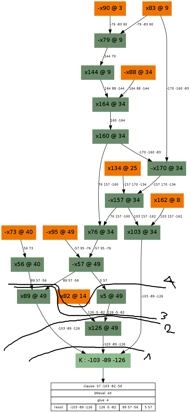
Our first implication graph had a clause “-70 55 42” (light green box) that caused a conflict — that is to say, somehow the variable setting {x70=TRUE, x55=FALSE, x42=FALSE} was set, the SAT solver realised that this is wrong, and something has to be done. Let’s look at what lead here! Guesses are coloured orange here, so it seems we made the following guesses during our SAT solving: x71=TRUE, x73 = FALSE, x42=FALSE. Now, we could just say, oh, well, setting x73 to FALSE was a dumb idea, just reverse that guess, and be done with it. That’s the easy (and the fast) way, but we are less lazy than that and we want to understand the reasons. So we do something called the conflict analysis to find something called an asserting clause that will not only let us reverse the guess x73=FALSE, but will also give the SAT solver a reason why that is a necessary assignment given its previous guesses and their consequences.

Consequences in the graph are coloured dark green, and there are exactly 3 of them: x70=TRUE, x55=FALSE and x56=TRUE. Each of these is a consequence of a clause that is in the SAT solver, marked on the edge(s) leading to it. For example, x56 is set to TRUE, because of the guess x73=FALSE and the clause “x56 V x73” marked on the edge leading to x56. A consequence that has one edge leading to it was propagated by a 2-long clause, a consequence that has 2 edges leading to it was propagated by a 3-long clause (e.g. consequence “x70=TRUE”, propagated by “x70 V x55 V x73”), etc. Okay, so how do we get to the reason? Well, we start out with the conflict, the clause “-x70 V x55 V x42” (at the bottom), and we do resolutions with this clause, going bottom up. We do as many resolutions as needed to reach the first UIP (also called “articulation vertex” or “dominator”), which is a unique point on the graph through which all paths go through from the highest decision level guess, in this case x73=FALSE, at decision level 56 (noted with a @56). If you take a look, the paths from x73=FALSE diverge from the very first point onwards, and there is no single point where they converge again. This means that the (first and only) dominator will be x73=FALSE itself, and we have to resolve with all clauses on the path:

  1. Start with clause “-x70 V x55 V x42”
  2. Resolve with clause “x70 V x55 V x73”
  3. Resolve with clause “-x55 V-x56 V -x71”
  4. Resolve with clause “x56 V x73”

This list is noted on the bottommost box’s lowest entry. When we resolve with these clauses, we are actually doing cuts on the graph, like this:

My drawing capabilities aren’t exactly great, but you can see that the cuts are successively higher and higher, until we reach the cut that has on its outer part the literals -x73, x71 and -x42. Unsurprisingly, exactly the inverse of these literals are what make up the final conflict clause. Now, if we unroll the implications until decision level 47 (but not the guess x42=FALSE), then with this clause added, variable x73 will propagate to TRUE automatically, essentially reversing the wrong guess — but also giving a reason why it needs to be reversed.

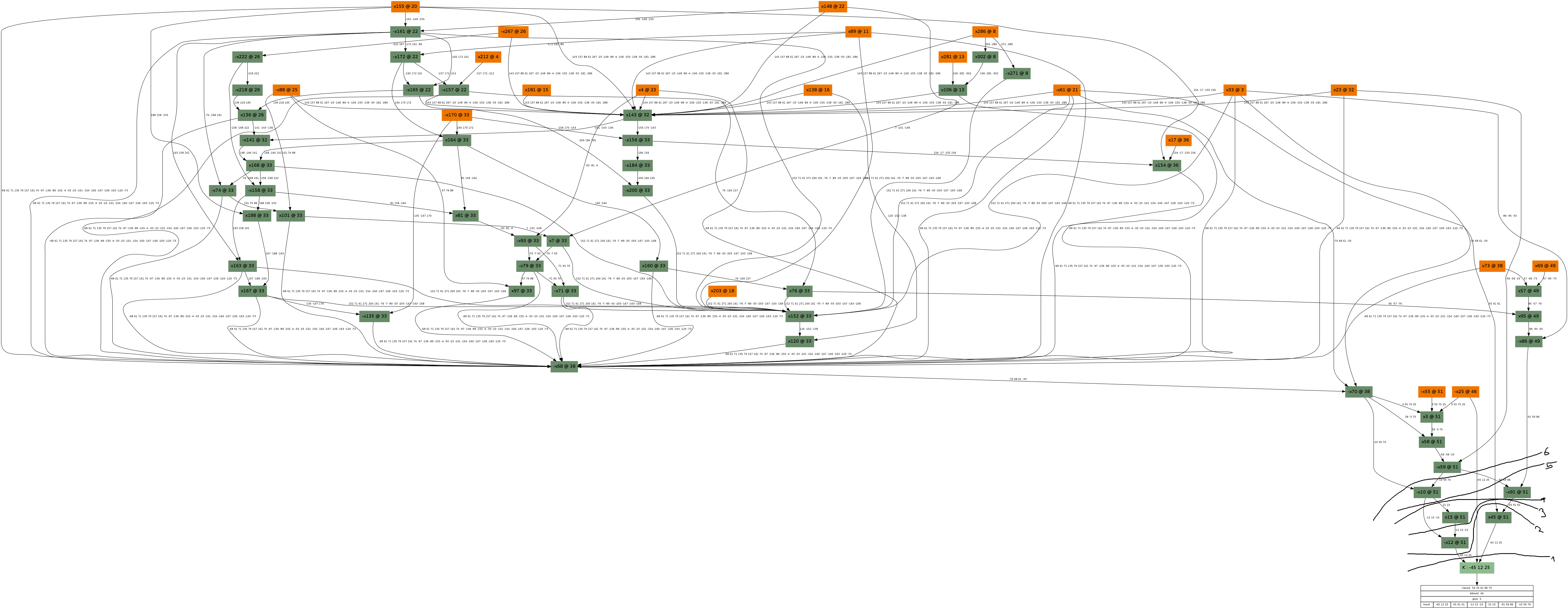
If you enjoyed the previous graph, here is another to entertain you further:

And its corresponding, not too obvious solution:

Note that I was too lazy to draw cuts 10, 11 and 12 around the assignment x145=FALSE (at decision level 39). The UIP in this case is again at the decision variable, x164. If you are still interested, here are some other examples:

PS: Thanks to George Katsirelos for his help understanding this (disclaimer: all faults belong to me alone).

Presentation at Hackito Ergo Sum

The HES’11 event was great: I had the pleasure of listening to some awesome presentations, and to meet some great people. The most interesting presentation from a non-technical point of view was the attacks at the automount feature of Linux, which everybody thinks is completely secure, but is in fact very flawed due to some buggy rendering libraries. It’s quite interesting that almost everyone thinks that their Linux installation is secure, when in fact if Linux was mainstream, viruses would be abound — but Linux is only a minor player, so malicious software is rarely written for it.

My presentation is available here. I tried mostly to demonstrate how SAT solvers work as an element of the technique that can most amply described as:

As the graphics show, the SAT solver is in fact only one player in this environment. As it turns out, it is the very last step after obtaining the cipher, creating equations describing the cipher, and converting the ANF equations into CNF. The best way to create equations from the original cipher is to use the excellent Sage Maths library for this, a tutorial of which is here. Then, the ANF created by Sage can be transcribed into CNF using, e.g. the anf2cnf tool by Martin Albrecht and me. Finally, the CNF must be solved with a SAT solver to recover the key of the cipher. This last step can be carried out by many SAT solvers, such as lingeling or MiniSat, but I prefer CryptoMiniSat, since I am the main developer for that SAT solver, and it is also very convenient to use in this domain due to some domain-specific advantages it has over other solvers. The middle two steps of the diagram are all automated by the Grain-of-Salt tool if you don’t want to use Sage, and it also contains some example ciphers, so you don’t even have to do step no. 1 in case you wish to work on one of multiple pre-defined industrial ciphers.

In case you are interested in the visualisations I used during my presentation, here is the set of tools I used. For the 3D visualisation, I used 3Dvis by Carsten Sinz — it’s a great tool to extract some structure from problems already in CNF. In case you still have the ANF, it contains more structure, though, and so it is more interesting to look at it that way. Unfortunately, that is rarely the case for typical SAT problems, and so one must often resort back to 3Dvis. For the example search tree, I used CryptoMiniSat 1.0 and gnuplot, and for the example real-time search, I used CryptoMiniSat 2.9.0, available from the same place. Unfortunately, CryptoMiniSat 2.9.0 cannot generate a search tree yet, but this eventually will be included, with time — especially if you join the effort of developing the solver. We are always looking forward to people joining in and helping out with various issues from graph generation to algorithm performance tuning, or even just some fun research.

Stats on CryptoMiniSat’s development

I have just discovered the gitstats tool, and quickly put together a set of statistics on the development of CryptoMiniSat, the SAT solver I have been working on lately. I have been using the GIT repository for most of my work on CryptoMiniSat, doing ~2000 commits since its inception, so it gives a good picture of how things evolved, and how I usually work. Firstly, the hours I usually work:

I basically work almost as much at midnight as I do at midday. The afternoon is clearly the most active and practically useful part of my day. Next, the graph to show which days I work the most:

Essentially, I worked as much on CryptoMiniSat during Sunday as I did during Monday or Friday. Saturday was the day I must have been the most fed up with development. Finally, the number of commits by months:

The 2nd and 3rd months of 2010 was a struggle because of the SAT and PoS deadlines. I tried to put together a credible research paper, which finally got accepted at PoS. During the 6th and 7th months of 2010 I was mostly looking forward to the results of the SAT Race, so I wasn’t developing so much.

Why programs fail

I just bought the book with the title of the blogpost by Andreas Zeller. Essentially, it’s about debugging, where the author analyses the chain of program defect leading to infected program state, finally leading to program failure. I bought the book because while working with CryptoMiniSat, I have encountered so many bugs that they could fill a book.

The problem with chasing bugs in CryptoMiniSat is that SAT solvers employ a very optimised algorithm that makes a lot of decisions per second, so recording all interesting events makes for a very big dump file. I have per-module verbosity settings, so if I can narrow down what module(s) are causing the failure, there is less debug output to go through, but sometimes I still have to wade through 10-20GB dumps to see how the program state got infected.

While going through such large dumps, the following occured to me: what if we loaded all this data into a MySQL database? Some 8 years ago I had a job where I processed a large chunk of the data on all of Hungary’s phone conversations on a daily basis. Essentially, data on your phone calls are recorded in many different databases, and these must be merged to calculate your bill and to provide statistical feedback to the company. I wrote a program that processed 3million records in about 1 hour using MySQL and a number of SQL statements that spanned approx. 2-3000 lines. In other words, I am not afraid of large databases, and I think such multi-gigabyte data could easily be loaded into a MySQL database.

The goal of loading a SAT run into a MySQL database is the following: once the MySQL data is ready, a bit of PHP, graphviz and gnuplot will plot any relevant information at any point in time about the solving. In other words, we could dig this data visually, with some very interesting effects.

For example, I have been lately having problems with clause strengthening interfering with variable elimination. The idea is in theory quite simple. Variable elimination eliminates a variable and adds clauses that represent the original clauses the variable was present in. These clauses are sometimes trivial, such as:
a or b or c or !c = true
which is never added since it is satisfied whether c is true or false. So far, so good. Clause strenghtening is a method whereby clauses are shortened. For example, if there was a clause:
e or b or c = true
the solver might discover that in fact it is also true that:
e or b = true
and replace the original clause with this, since this clause is “stronger”: it poses a more stringent requirement. The way variable elimination and clause strenghtening interact is as follows. Let’s suppose we eliminate on varible e. If the above clause is strenghtened before elimination, then instead of:
a or b or c or !c = true
we might have got:
a or b or !c = true
which must be added. We actually have more clauses because of clause strenghtening! I believe nobody ever found this anomaly. To properly quantitise how this affects solving, we need to know all states of a clause, and a web interface with a MySQL backbone could help a lot with that.